
Superconducting Qubit (Elementary Ver.)
Author:Peir-Ru Wang
\(\to\)中文版
Update
(11)2025.02.07:QPU Topology
(10)2025.02.06:Superconducting Qubits under Electron Microscopy
(09)2025.02.05:Other Types of Qubits
(08)2025.02.04:What Does a Superconducting Quantum Computer Look Like?
(07)2025.02.03:Modern Mainstream Superconducting Qubits
(06)2025.02.02:Overview of Superconducting Circuit Qubit Types
(05)2025.02.01:How Are Signals Delivered to Qubits?
(04)2025.01.24:Early Types of Superconducting Qubits
(03)2025.01.12:What is a Superconducting Qubit?
(02)2025.01.10:Josephson Junction
(01)2025.01.06:Topic Establishment
- Josephson Junction
- What is a Superconducting Qubit?
- A Brief Overview of Superconducting Circuit Qubit Types
- Qubits based on superconducting circuits using Josephson Junctions, sometimes referred to as artificial atoms. A single qubit size is about the micrometer (\( \mu m \)) scale. This article focuses on this type of qubit.
- Topological qubits, using superconductors as the substrate, with nanowires placed on the surface. Due to the proximity effect, the nanowires are influenced by the substrate's superconductivity. Applying a magnetic field to break time-reversal symmetry forms special Majorana states at both ends of the nanowires. This topic may be discussed in the future. \(^a\)
- Type A: A1 represents a single Josephson Junction (JJ) as a qubit, an earlier qubit design.
- Type B: A2–A8, based on a single JJ shunted with a capacitor (C-shunt). Later designs aimed to increase coherence time by connecting large inductors in parallel or reducing capacitance to mitigate noise effects.
- Type C: A9–A10, qubits with modifications on one side of the JJj, making the ground state phase difference non-zero. These can be achieved through complex circuit designsa,b,c, replacing the insulating layer with magnetic materialsd,i, or using s-wave with d-wave heterostructure JJsg,h.
- Type Hybrid: A11, representing superconducting qubits combined with spin quantum dots (Spin Quantum Dot, Spin QD)k. Other types include combinations with superfluid heliume,f, ion traps, and more.l
- Early Types of Superconducting Qubits
- Current Mainstream Types of Superconducting Qubits
- Superconducting Qubits Under Electron Microscopy
- Other Types of Qubits
- What Does a Superconducting Quantum Computer Look Like?
- Frequency control *1: The flux line for tuning magnetic flux.
- State control *1: The drive line.
- State readout *2: One input and one output readout line.
- How Are Signals Delivered to Qubits?
- QPU Topology
- How to Control a Superconducting Qubit
- Pulse Amplitude (\( A \)): Determines the state of the Qubit (the rotation angle on the Bloch sphere)
- Pulse Duration (\( T \)): Determines the state of the Qubit (the rotation angle on the Bloch sphere)
- Pulse Frequency (\( \omega_d \)): Ensures precise driving of the Qubit
- Pulse Envelope (\( F(t, \tau) \)): Affects leakage
Superconducting qubits are fundamentally based on the Josephson Junction. A Josephson Junction is a sandwich-like structure consisting of two superconductors separated by a non-superconducting material. Due to quantum tunneling, superconducting current can pass through the non-superconducting layer. Commonly used materials are aluminum-based (Al) or niobium-based (Nb). A Josephson Junction can be fabricated by first depositing a superconducting metal layer on a substrate, allowing it to oxidize and form a thin insulating oxide layer (the non-superconducting layer), and then depositing another superconducting metal layer. This Superconductor-Insulator-Superconductor structure is known as an SIS junction.
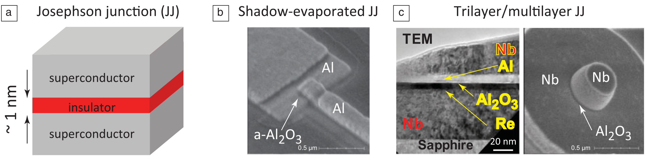
▲ (a) Schematic of an SIS Josephson Junction. (b) Electron microscope image of an aluminum-based SIS junction. (c) The superconducting critical temperature \(T_c = 1.2K\) for aluminum, while niobium has the highest \(T_c = 9.2K\) among single-element superconductors. Therefore, using niobium can provide better stability for qubits. However, the structural difference between niobium oxide (\(Nb_2O_5\)) and metallic niobium makes it difficult to produce high-performance Josephson Junctions. Hence, a multilayer structure \(Nb-Re-Al_2O_3-Al-Nb\) is used, where alumina serves as the insulating layer, and thin \(Re\) and \(Al\) layers act as buffer layers. This buffer technique, common in modern semiconductor manufacturing (heterogeneous integration), involves using two or three atomic layers to bridge the mismatch between two materials with different lattice constants. Another well-known quantum effect in quantum materials is the proximity effect, where the wave function of the bulk material fully penetrates the thin film layer, effectively transforming the thin film's properties into those of the bulk material. Due to the proximity effect, the buffer layer also becomes superconducting, making this multilayer structure an SIS junction.
Ref: 10.1557/mrs.2013.229
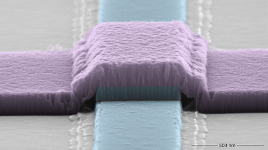
▲ Example of a niobium-based Josephson Junction
Ref: David Schuster of Stanford University
https://www.anl.gov/article/resurrecting-niobium-for-quantum-science
https://schusterlab.stanford.edu/research.html
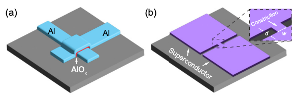
▲ Quantum effects are fragile. In fact, Josephson Junctions are highly sensitive, and fabricating a well-insulated layer that is perfectly integrated into the sandwich structure is extremely challenging. Any defects in the structure can lead to qubit decoherence and errors. Therefore, scientists continuously explore alternative solutions. Figure (b) shows a theoretical proposal using constriction, where local superconductivity is lost naturally, forming a Josephson Junction (ScS).
Ref: 10.1103/PhysRevA.110.012427
https://quantumzeitgeist.com/superconducting-qubits-get-boost-with-novel-constriction-design/
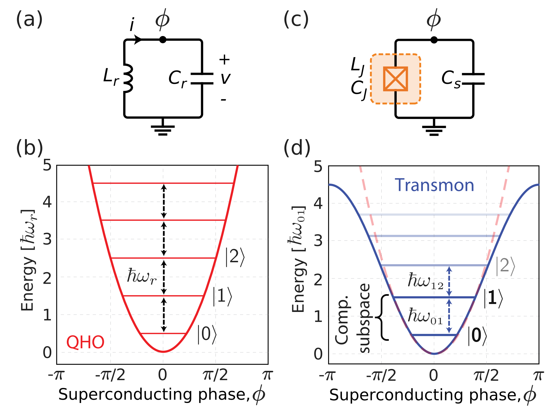
In classical computing, a series of classical bits records information using two states, 0 or 1. Similarly, quantum bits (qubits) record information and perform computations using different quantum states. The simplest concept of quantum energy levels is the Quantum Simple Harmonic Oscillator. To implement a simple harmonic oscillator using an electronic circuit, the simplest approach is an \( LC \) circuit, composed of an inductor \( L \) and a capacitor \( C \), as shown in figure (a). In classical physics, the harmonic oscillator is continuous, but in the quantum world, energy levels are discrete. Different energy levels can be used to encode information, and we typically represent these levels using \( \ket{0} \), \( \ket{1} \), \( \ket{2} \)... or \( \ket{g} \), \( \ket{e} \), \( \ket{f} \)... to denote different energy states, as shown in figure (b). In figure (b), it is evident that the energy gap between each level is the same, \( \hbar \omega_r \). However, when we want to operate a qubit, we prefer the system to be limited to transitions between \( \ket{0} \) and \( \ket{1} \) only. This requires a nonlinear component to distinguish between \( \ket{0} \), \( \ket{1} \), and the unwanted higher energy levels. The Josephson junction is a highly effective nonlinear inductive element, as shown in figure (c). In figure (d), we can see that the energy gaps become unequal, allowing us to utilize this property to operate the qubit. Therefore, the most basic superconducting qubit consists of a superconducting capacitor and a Josephson junction!
Ref: 10.1063/1.5089550
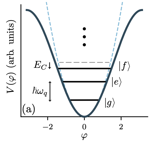
▲ This figure clearly shows the energy level changes in a superconducting qubit. The second excited state \( \ket{f} \) (or \( \ket{2} \)) has lower energy.
Ref: 10.1103/RevModPhys.93.025005
Superconducting-based quantum bits can be classified into two main types:
Superconducting circuits made of Josephson Junctions can refer to the figure below, showing different superconducting qubit types:
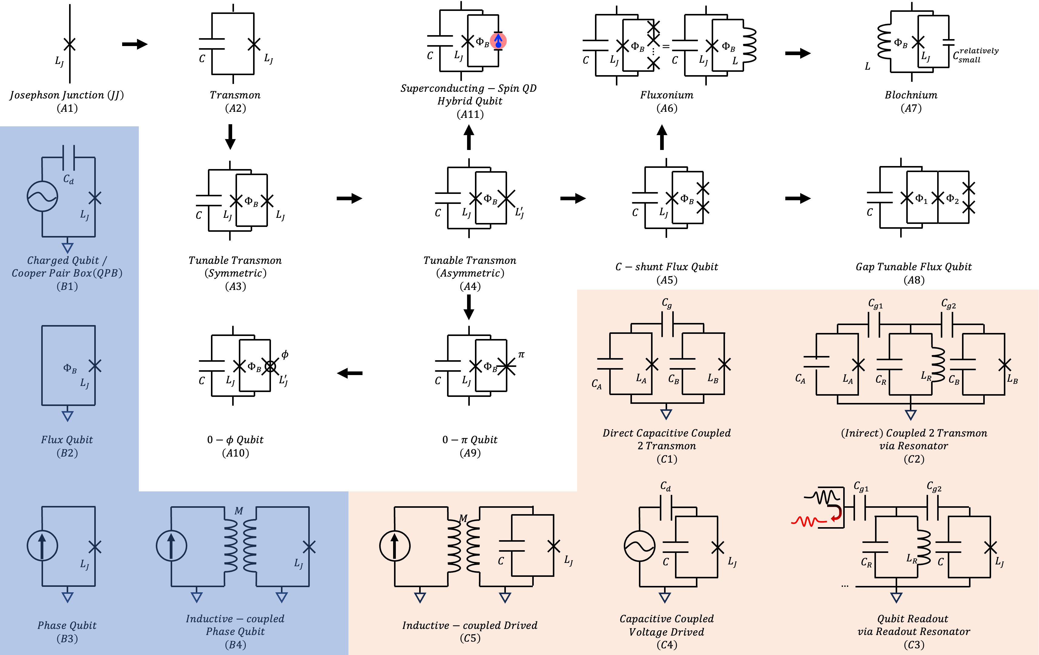
The A series represents the most basic unit to form a single qubit. The arrows indicate the conceptual extension directions. I categorize them into four main types:
\(^b\)10.1088/1367-2630/aab7cd
\(^c\)10.1088/1367-2630/ab09b0
\(^d\)10.1038/s43246-024-00659-1
\(^e\)10.1103/PhysRevA.101.012336
\(^f\)10.1038/s41467-019-13335-7
\(^g\)10.1109/TASC.2019.2892078
\(^h\)10.1088/1361-6668/ab7053
\(^i\)10.1103/PhysRevApplied.8.054028
\(^j\)10.1088/0953-2048/21/3/034011
\(^k\)10.1038/s41567-023-02071-x
\(^l\)arXiv: 1204.2137
(A8) https://www.ntt-review.jp/archive/ntttechnical.php?contents=ntr201209fa2.html
The B series represents examples of Type A qubits paired with control circuits, using different control circuit techniques. More details can be found in Early Types of Superconducting Qubits.
The C series represents examples of Type B qubits paired with control circuits.
Almost all superconducting qubits are based on Josephson Junctions, combined with capacitors and inductors. Early superconducting qubits can be categorized as shown in the figure below:
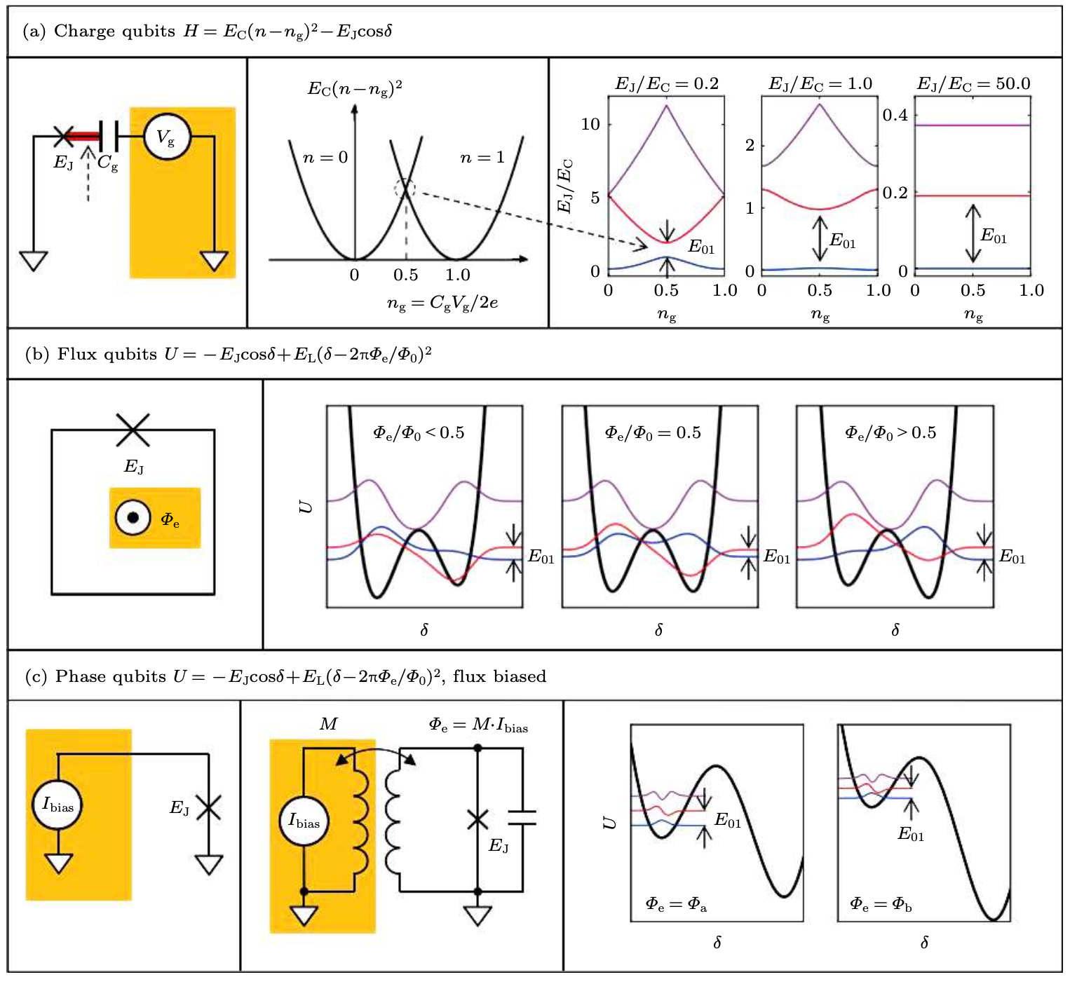
▲ Early superconducting qubits are divided into three main types: Charge Qubit, Flux Qubit, and Phase Qubit. The simple conceptual differences lie in the primary methods of controlling the qubits (highlighted in yellow boxes in the figure):
\(\to\) (a) Controlled by voltage: Voltage alters the stored charge in the capacitor, referred to as a Charge Qubit.
\(\to\) (b) Controlled by magnetic flux: Magnetic flux alters the energy storage in the Josephson Junction, referred to as a Flux Qubit.
\(\to\) (c) Controlled by induced current: Induced current alters the phase of the Josephson Junction, referred to as a Phase Qubit.
Ref: 10.7498/aps.71.20211865
The evolution of early superconducting qubits can be observed in the figure below:

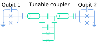
Early superconducting qubits were highly susceptible to noise and relied on external control circuits to form energy levels. These external control circuits often consisted of large control instruments (referred to as "large" relative to the micrometer-scale JJ, imagine them being the size of everyday computers, with characteristic dimensions in centimeters). Such large integrated circuits introduced significant classical noise, leading to qubit decoherence. To improve fidelity, a capacitor (\(C\)) was connected in parallel, forming what is known as a Transmon. A single Transmon constitutes an \(LC\) circuit with quantized energy levels.
Because Transmons have their quantum frequencies, precise frequency control and resonance are required to alter their quantum states for quantum computation. When developing large-scale quantum circuits, a single control or readout line often connects multiple qubits. If their frequencies are too similar, signals may interfere with adjacent qubits in the spectrum, causing crosstalk. Frequency adjustments are achieved by altering the capacitance value (\(C\)) or the inductance of the Josephson Junction (\(L_J\)) during fabrication. However, precise control of frequency isolation between qubits during fabrication is extremely challenging. Manufacturing errors can lead to deviations, and once fabrication is complete, adjustments cannot be made, lowering the yield. Moreover, over time (e.g., monthly or daily), the frequency of Josephson Junctions deviates from their original design due to atomic or defect diffusion at the heterogeneous material interface. Once the deviation exceeds a threshold, the entire circuit fails. Thus, the importance of "post-fabrication frequency tuning" for Transmons becomes evident. Scientists use two JJs forming a SQUID to create a Tunable Transmon, where magnetic flux between the two JJs can adjust the Transmon's frequency. This enables synchronization of qubit calibration during computation, achieving frequency isolation. The dual JJs in a Tunable Transmon can be symmetric (identical) or asymmetric (different). Symmetric designs allow a wider tunable frequency range but are more affected by noise in magnetic flux control; asymmetric designs, while having a smaller tunable range, offer higher frequency stability.
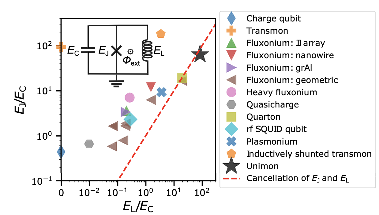
While a Transmon eliminates reliance on external control instruments, adding a capacitor (\(C\)) introduces stored energy by separating positive and negative charges. This creates a micrometer-scale dipole, making it highly susceptible to electromagnetic noise, causing decoherence. To mitigate this, scientists focus on one side of the Josephson Junction and replace it with multiple series-connected JJs to form an inductor (\(L\)), called Fluxonium. Fluxonium currently achieves decoherence times in the microsecond range.
Further improvements in qubit stability focus on continuously increasing inductance (\(L\)) and reducing capacitance (\(C\)), leading to developments like Blochnium. The following figures illustrate that different superconducting qubits essentially involve tuning \(L\), \(C\), and \(J\).
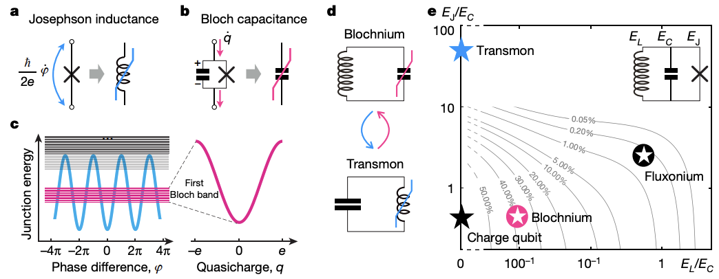
▲ The right side of this figure illustrates the duality of the Transmon and Blochnium concepts. The Transmon is a "nonlinear inductor" paired with a capacitor, while Blochnium can be seen as a "nonlinear capacitor" paired with an inductor.
Ref: 10.1038/s41586-020-2687-9
Ref: ar5iv.labs.arxiv.org/html/1907.02937
Ref: 10.1038/s41467-022-34614-w
arxiv.org/pdf/2106.11352
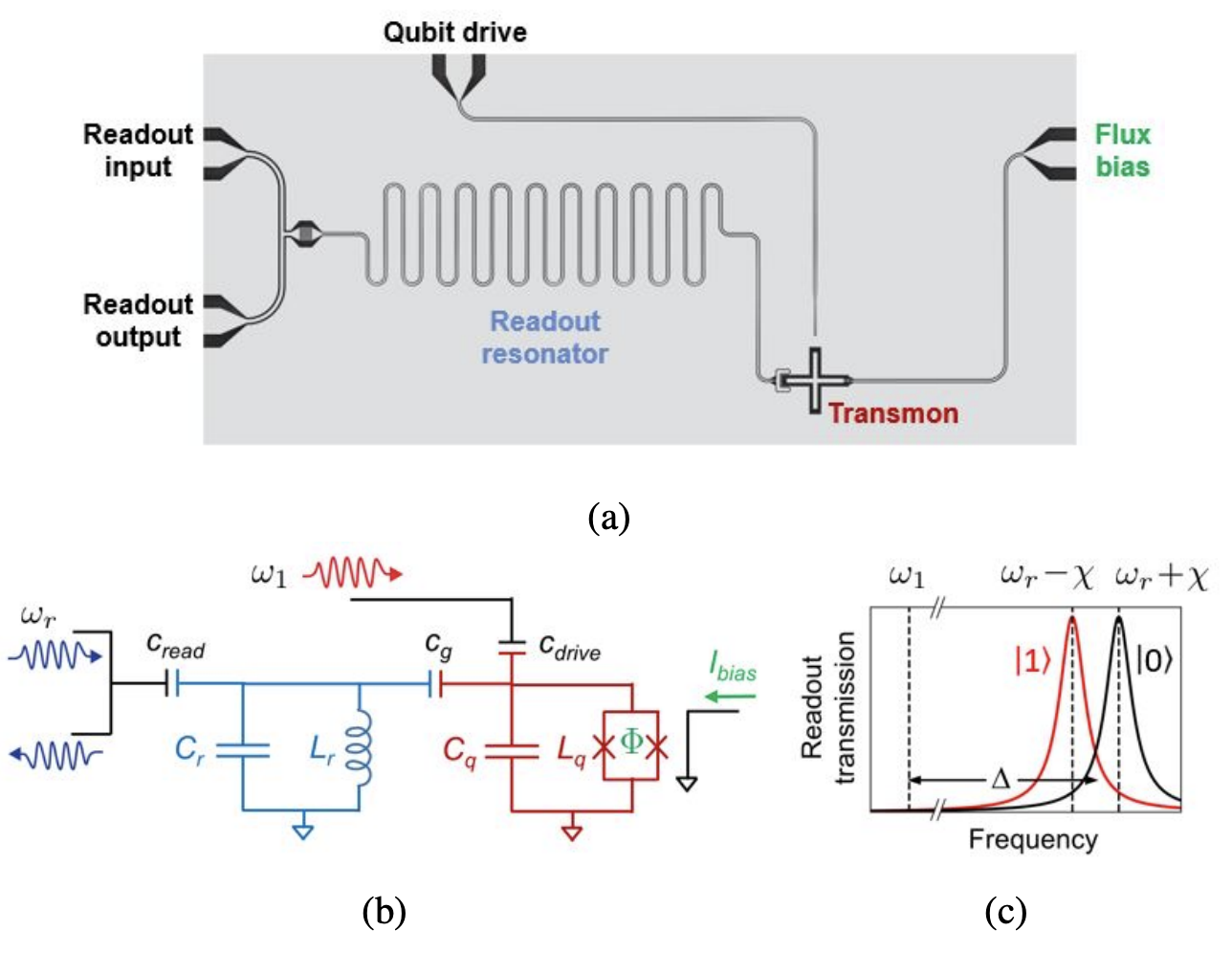
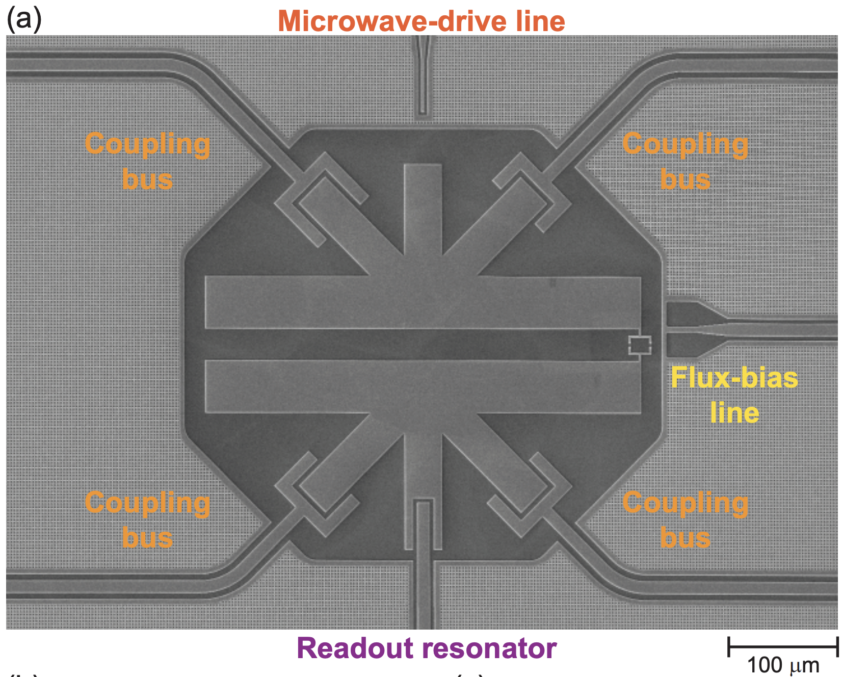
▲ Take a look at the layout of a Transmon. (a) shows the circuit layout under a microscope, and (b) provides the corresponding circuit diagram. In this figure, there is a Qubit (red Transmon), a readout resonator (light blue), and two feedlines, one driving the qubit and the other driving the readout resonator. Components are coupled through capacitors. Additionally, a flux line connected to the Qubit generates a magnetic field to adjust the Transmon's operational frequency. (c) The readout resonator, coupled with the qubit, undergoes frequency shifts depending on whether the qubit is in state \(|0\rangle\) or \(|1\rangle\). This frequency shift characteristic of the readout resonator is used to determine the qubit's state.
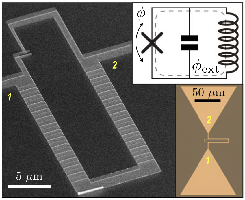
▲ On one side of the Josephson Junction, multiple JJs are connected in series to form an inductor (\(L\)), referred to as Fluxonium.
Ref: 10.1038/s41467-021-26686-x
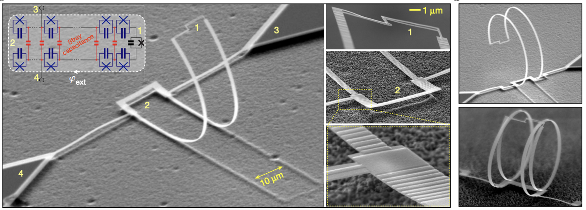
▲ Blochnium can be viewed as an advanced Fluxonium, with its inductor further constructed by connecting more Josephson Junctions in series. Its three-dimensional structure is intriguing.
Ref: 10.1038/s41586-020-2687-9
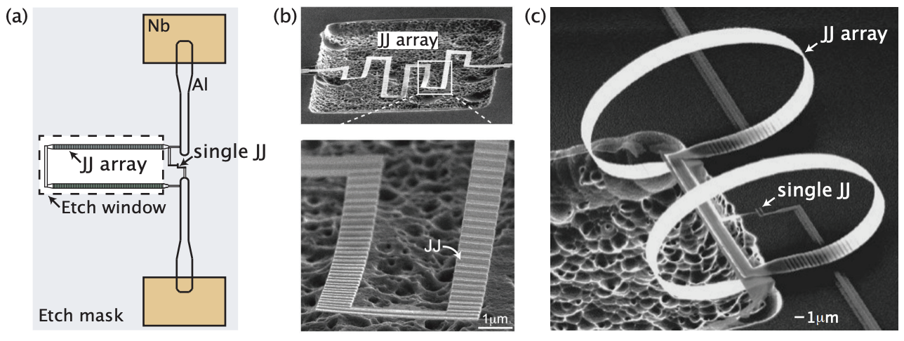
▲ Another image of Josephson Junction arrays in the etching process for Fluxonium/Blochnium. This clearly shows that the squid-like structure is formed by a series of Josephson Junctions.
Ref: arxiv: 2411.10396
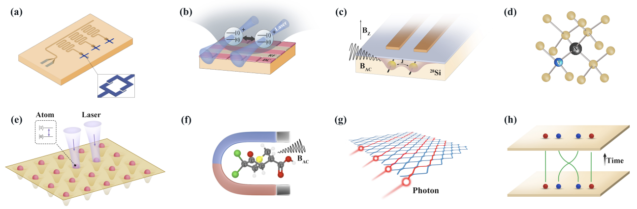
Previous discussions covered composite superconducting qubits. Here, we briefly introduce other types of qubits. In applications, qubits must strike a balance between easy controllability and resistance to noise, extending decoherence time. However, these two demands often conflict; ease of control means greater susceptibility to noise, while higher stability implies difficulty in control.
Developing hybrid systems that integrate different qubit types or composite qubits is a viable direction.
Ref: arxiv: 2303.04061
(a) Superconducting Quantum Processor
Composed of artificial atom arrays using Josephson Junctions and capacitors, controlled via microwave electronics.
Qubit Count: ~100
Quantum Gate Fidelity:
Single Qubit Gate \(F_1 > 99\%\), Two Qubit Gate \(F_2 > 99\%\)
Pros: Fast operation, high controllability, excellent scalability
Cons: Crosstalk, low-temperature requirement, challenges in large-scale expansion
(b) Trapped Ion Quantum Computing
Utilizing laser-cooled atomic ions, trapped with RF electric fields and manipulated with lasers.
Qubit Count: 20–30
Quantum Gate Fidelity:
Single Qubit Gate \(F_1 > 99.9\%\), Two Qubit Gate \(F_2 > 99\%\)
Pros: Long coherence time, high gate precision, reconfigurable qubit links
Cons: Difficult to scale up technically
(c) Semiconductor Spin-Based Quantum Computing
Utilizing the electron or hole spin within semiconductor quantum dots as qubits.
Qubit Count: 6
Quantum Gate Fidelity:
Single Qubit Gate \(F_1 \approx 99.99\%\), Two Qubit Gate \(F_2 \approx 99.5\%\)
Pros: Mature technology, long coherence time, compact footprint
Cons: Requires nanoscale manufacturing precision
(d) NV Center Quantum Computing
Quantum operations using the long coherence time of electron and nuclear spins at point defects in diamonds (NV centers).
Qubit Count: 10
Quantum Gate Fidelity:
Single Qubit Gate \(F_1 \approx 99.995\%\), Two Qubit Gate \(F_2 \approx 99.2\%\)
Pros: Room-temperature operation, high sensitivity, suitable for quantum networks
Cons: Difficult to scale up
(e) Neutral Atom Array Quantum Computing
Utilizing optical tweezers to trap neutral atoms and controlling interatomic interactions via Rydberg effects.
Qubit Count:
Digital Processor: 24
Analog Simulator: 289
Pros: Supports both digital computation and analog simulation, highly scalable
Cons: Needs improvement in two-qubit gate fidelity
(f) NMR Quantum Computing
Using nuclear spins in molecules for quantum operations.
Qubit Count: 12
Quantum Gate Fidelity:
Single Qubit Gate \(F_1 \approx 99.98\%\), Two Qubit Gate \(F_2 \approx 99.3\%\)
Pros: Room-temperature operation, long coherence time, suitable for digital simulations
Cons: Difficult to scale up to large systems
(g) Photonic Quantum Computing
Manipulating quantum information using single photons or conjugate variables of electromagnetic field modes.
Qubit Count: 18 (individual control), 255 (Jiuzhang 3.0)
Quantum Gate Fidelity:
Single Qubit Gate \(F_1 \approx 99.84\%\), Two Qubit Gate \(F_2 \approx 99.69\%\)
Pros: Resistance to decoherence, room-temperature operation, suitable for distributed quantum computing
Cons: Photon-photon gates are challenging to implement
(h) Topological Quantum Computing
Based on topological encoding using non-Abelian anyons, performing operations through braiding.
Qubit Count: Experimental stage
Quantum Gate Fidelity: N/A
Pros: Intrinsic topological protection, potential for large-scale error correction
Cons: Still in development
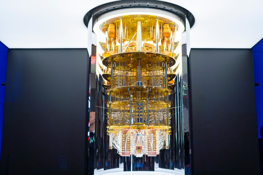
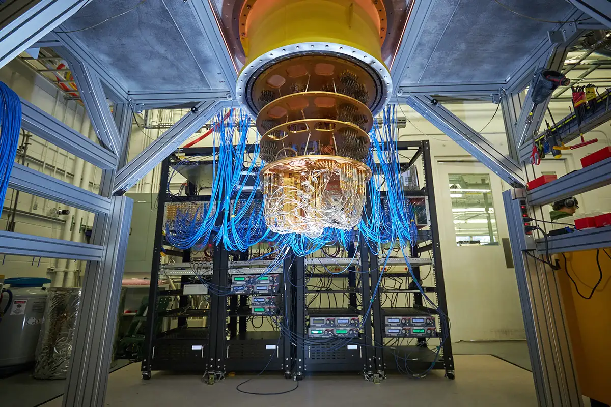
A complete superconducting quantum computer must include a helium-3 ultra-low temperature vacuum environment, a cooling system, and numerous RF signal control and readout instruments. Hence, current superconducting quantum computers are extremely large. Additionally, each qubit requires at least four lines:
https://arxiv.org/pdf/1612.08208
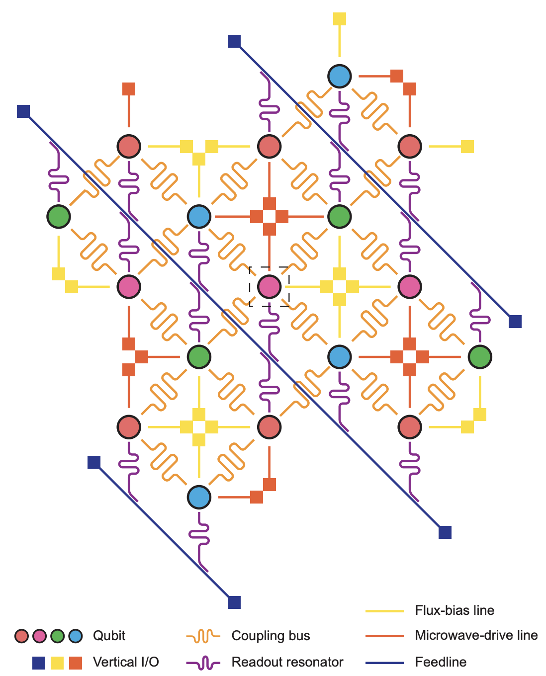
▲ Quantum computation requires operating numerous qubits simultaneously, along with additional qubits for error correction. The image above shows a 17-qubit experimental quantum chip arranged in a type of quantum error correction layout called surface code. Pink and red denote data qubits, while light blue and green indicate check qubits. Each qubit connects to seven lines (nicknamed Starmon), including four coupling lines, one flux line, one drive line, and one readout resonator. The readout resonators are integrated into three feedlines. Although current technology allows multiple qubits to share a readout line via frequency isolation, we still need to consider resonators for inter-qubit interaction. A prototype 100-qubit quantum computer requires around 400 external lines, making superconducting quantum computers densely wired.
arxiv: 2408.12433
Resonators or couplers for inter-qubit interactions can be tunable, enabling adjustment of coupling strength between qubits. However, this also increases the complexity of the control circuit.
Ref: IBM
Ref: Google
Ref: IQCC and Quantum Machines
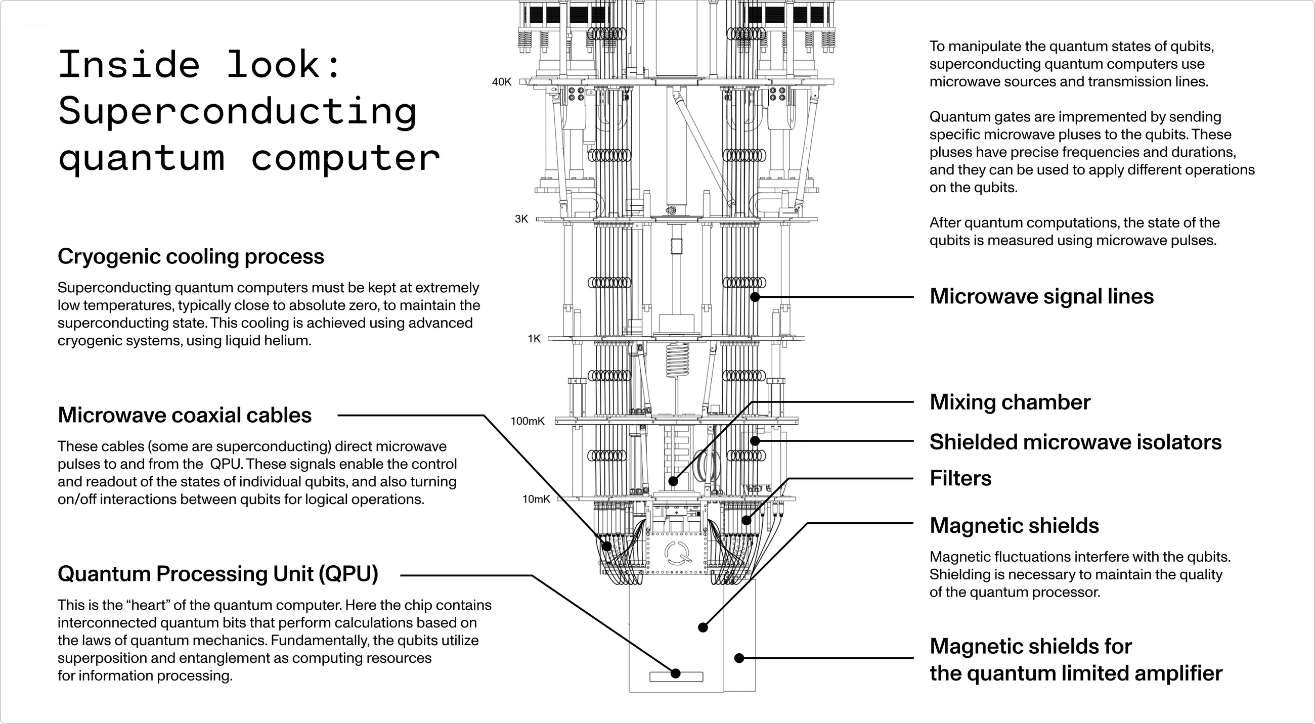
▲ IQM illustrates detailed designs of the quantum computer's cryogenic chamber.
Ref: IQM
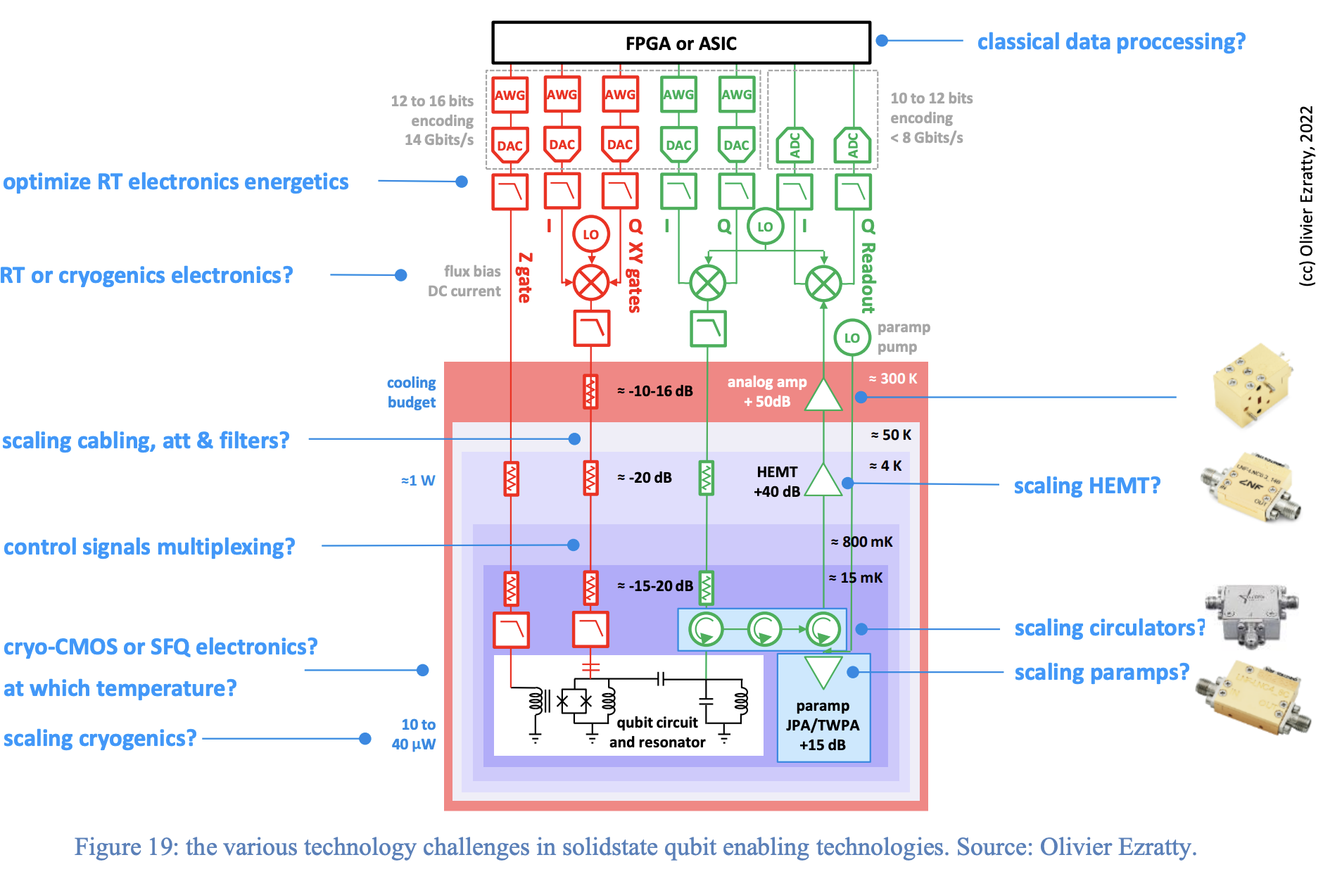
In the previous section, we discussed the complex hardware design of quantum computers. Here, we briefly explain the signal delivery system for controlling superconducting quantum computers. Control signals are generated by arbitrary waveform generators (AWG) as digital signals, converted to analog signals via digital-to-analog converters (DAC), filtered through multiple layers, and then sent to the quantum circuit. Feedback signals are converted back to digital signals using analog-to-digital converters (ADC) for measurement.
Ref: arxiv: 2303.15547
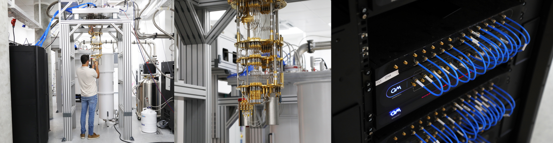
The images above illustrate the complex layers of wiring passing through the cryogenic chamber into the qubits. Designing such intricate wiring while ensuring noise reduction and thermal isolation increases costs and error rates, making scalability challenging. Below are two potential solutions to reduce the number of wires:

▲ Fiber optic solution: (a) shows traditional control wiring, while (b) demonstrates the use of wavelength-multiplexed carrier signals. Control signals are sent via fiber optic bundles into the chamber after being converted into corresponding carriers by optical-electrical converters.
Ref: DOI: 10.1038/s41586-021-03268-x
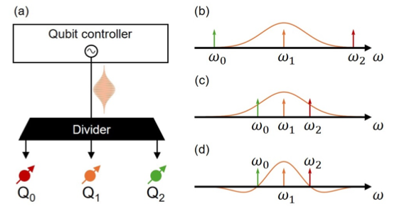
▲ By isolating qubit frequencies and designing specific control spectrum signals, multiple qubits can be controlled via a single control line.
Ref: arXiv:2501.10710v1
Here, we briefly discuss QPU (Quantum Processing Unit) design. Current quantum circuits are two-dimensional, with inter-qubit interactions typically limited to neighboring qubits. Coupled with common error correction designs (QEC), such as the surface code, which adopts a square design, each QPU qubit only needs four couplers for neighboring qubits. IQM has also proposed new QPU designs incorporating computational resonators to enable more advanced quantum computing methods. We may write more about this in the future.
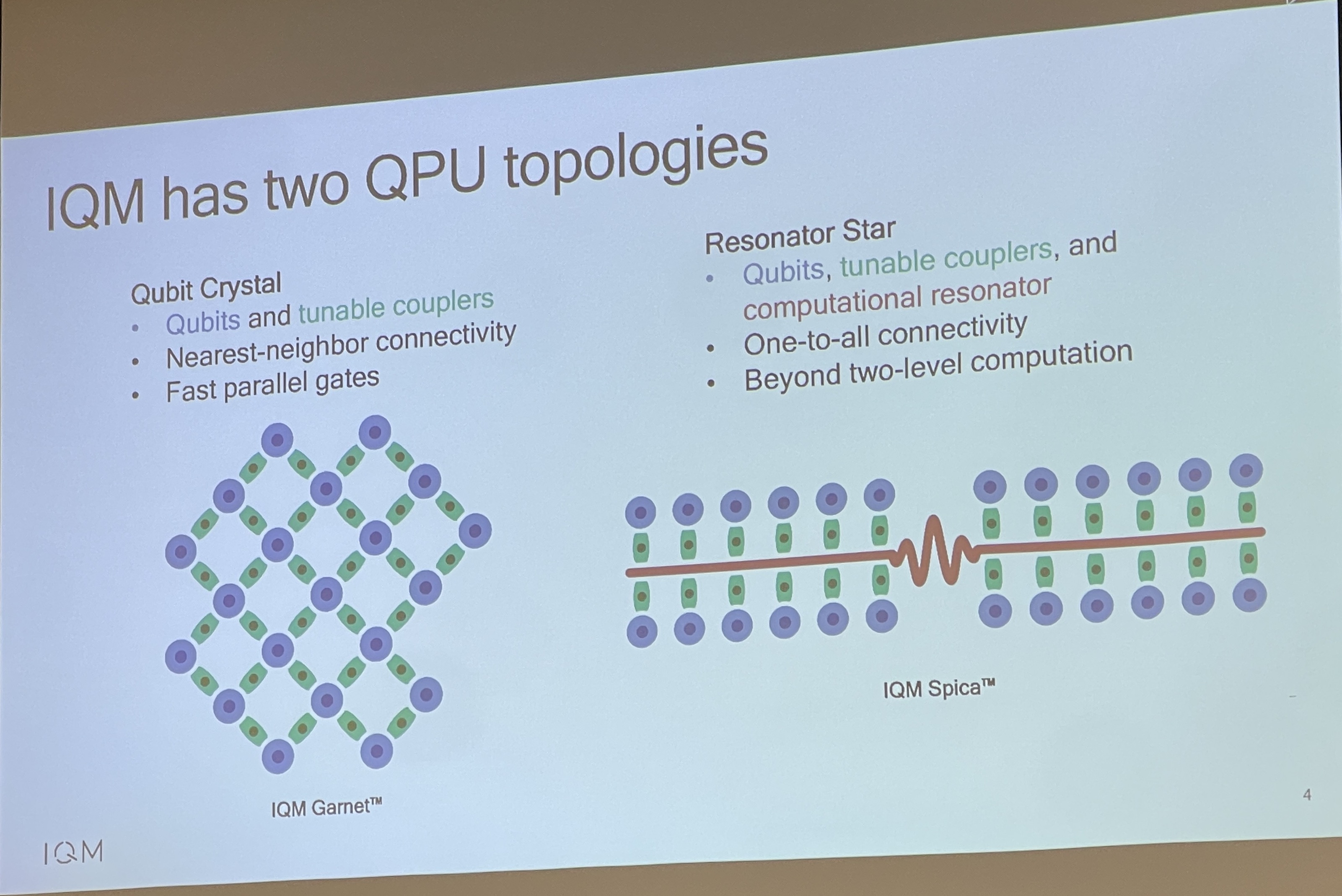
Ref: IQM
Ref: arXiv: 2408.12433
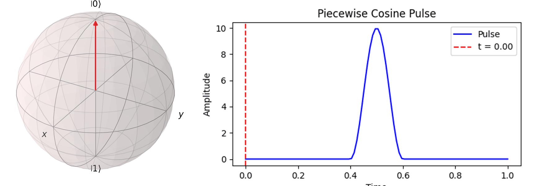
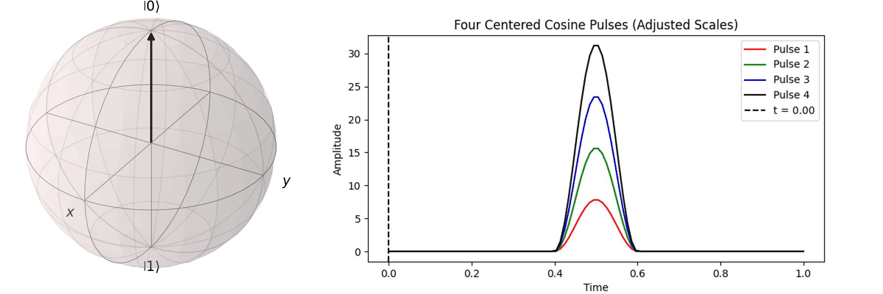
The most common method is Rabi oscillation, achieved by applying an oscillating pulse \( P(t) \) with a specific frequency. Let’s first visualize a Qubit undergoing a \( \pi \)-pulse transition from \( |\ 0\rangle \rightarrow |\ 1\rangle \) using the Bloch sphere:
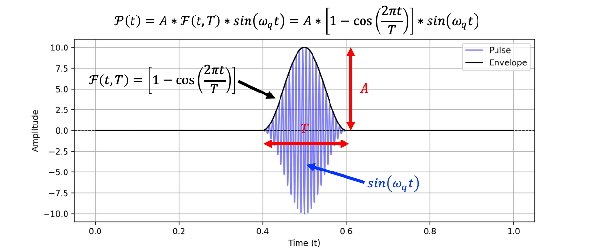
Main Parameters for Controlling a Qubit
A complete pulse can be expressed as: \[ P(t) = A \cdot F(t, \tau) \cdot \sin(\omega_q t) \]
Here’s an example:
Generally, because the coherence time of a Qubit is very short, we aim to complete Qubit operations as quickly as possible. For superconducting qubits, the coherence time can reach microseconds (\(\mu s\)), which is already considered long in current technology. Therefore, pulses for superconducting qubits are typically in the nanosecond (\(ns\)) range. Consequently, the Qubit state is usually controlled by adjusting the pulse amplitude to determine the rotation angle.
(For example, in the experiment from DOI: 10.1103/PRXQuantum.5.030353, the driving duration is approximately \( 10ns \)).
The process can be visualized using the Bloch sphere, as shown here for rotations around the \( X \)-axis by \(0.25\pi\), \(0.5\pi\), \(0.75\pi\), and a full \( \pi \)-pulse. It can be observed that the rotation angle is determined by the pulse amplitude.
Similarly, we can discuss achieving the same \( \pi \)-pulse transition from \( |\ 0\rangle \rightarrow |\ 1\rangle \) using different pulse durations (\( T \)).
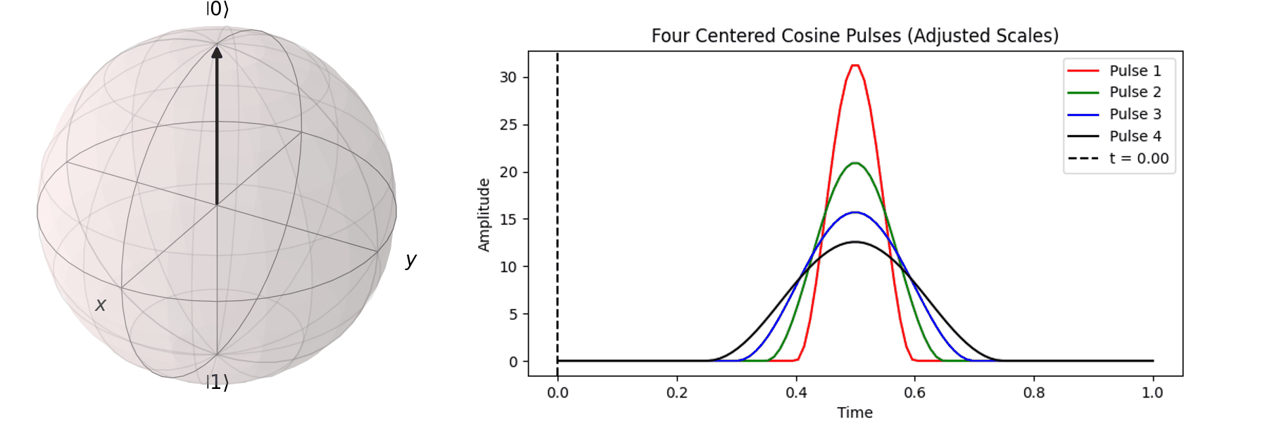
Naively, one might think that since superconducting qubits have a short coherence time, the shorter the pulse duration (\( T \)), the better. In the next section, we will discuss how shorter pulses introduce more irrelevant oscillation frequencies, leading to errors in Qubit operations. In practice, determining the appropriate pulse duration (\( T \)) and amplitude (\( A \)) is a crucial part of regular Qubit calibration. Good calibration ensures high-quality quantum computation, whereas poor calibration can result in errors that make quantum computation less accurate than classical computation.
後記
Index
Contact:
![]()