SC Qubit

Author:Peir-Ru Wang
\(\to\)Chinese Version
Update
(O04)2025.02.07：New-Computational Science and Two-Level Systems (TLS)
(O03)2025.01.18：New-Coupling Between Two LC Circuits
(O02)2025.01.12：New-Driving an LC Circuit
(O01)2024.12.29：New-New web

Basics of Quantum Computing Hardware

Quantum computing demonstrates immense computational potential in specific problems compared to classical computers. However, its hardware faces challenges such as difficulty in control and short operation times. Quantum computing hardware revolves around quantum bits (qubits) as core components, supplemented by driving components to manipulate qubit states and readout components to measure them. Furthermore, due to qubits' susceptibility to external interference, calibration/adjustment components and quantum error correction components are also necessary. In summary, they can be categorized as follows:

Qubits
Driving components
Readout components
Calibration components
Error correction components

In fact, current memory systems also include similar hardware divisions, but in quantum computing, these components need to be considered holistically. More specifically, due to interactions between different components, when quantum physics is employed to describe the entire quantum circuit using its Hamiltonian (or Schrödinger equation), the interactions will "modify" the properties of qubits. On one hand, these modifications enable the operation and measurement of qubit information; on the other hand, they cause deviations from ideal states, leading to errors.

This article focuses on superconducting quantum circuits, with the components in quantum circuits categorized as follows (from two perspectives):

From a functional perspective	1. Qubits (Data storage) 2. Driving components: Coupling circuits or LC resonators (for computation) 3. Readout components: LC resonators and feedlines 4. Calibration components: Flux lines (to adjust qubit frequencies) 5. Error correction components: Qubits (used for error correction)
From a component perspective	1. LC Circuits a. LC resonators (linear LC circuits): Used for reading qubit states (readout resonators) and sometimes for indirect coupling between qubits b. Qubits (nonlinear LC circuits): Partly for data storage, partly for error correction 2. feedlines: Delivering and receiving external signals 3. Coupling components: a. Operating and changing qubit states b. Direct coupling between qubits c. Exchanging signals between external sources and components 4. Flux lines: Adjusting qubit frequencies to ensure qubits operate at specific frequencies

From a functional perspective

1. Qubits (Data storage)
2. Driving components: Coupling circuits or LC resonators (for computation)
3. Readout components: LC resonators and feedlines
4. Calibration components: Flux lines (to adjust qubit frequencies)
5. Error correction components: Qubits (used for error correction)

From a component perspective

1. LC Circuits
   a. LC resonators (linear LC circuits): Used for reading qubit states (readout resonators) and sometimes for indirect coupling between qubits
   b. Qubits (nonlinear LC circuits): Partly for data storage, partly for error correction

2. feedlines: Delivering and receiving external signals

3. Coupling components:
   a. Operating and changing qubit states
   b. Direct coupling between qubits
   c. Exchanging signals between external sources and components

4. Flux lines: Adjusting qubit frequencies to ensure qubits operate at specific frequencies

arxiv.org/pdf/2106.11352
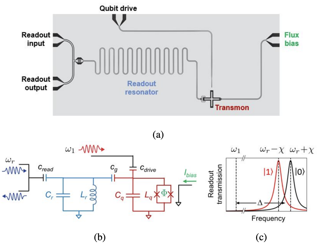
Let's first take a look at the layout of a single qubit. (a) A microscope view of the circuit, (b) the corresponding circuit diagram. This diagram includes a qubit (red transmon), a readout resonator (light blue), and two feedlines separately driving the qubit and the readout resonator. Components are coupled via capacitors. Additionally, a flux line near the qubit generates a magnetic field to adjust the operational frequency of the transmon. (c) The readout resonator, coupled to the qubit, shows spectral shifts depending on whether the qubit is in state \(|0\rangle\) or \(|1\rangle\). This spectral shift allows determination of the qubit state.

doi.org/10.1038/nature08121
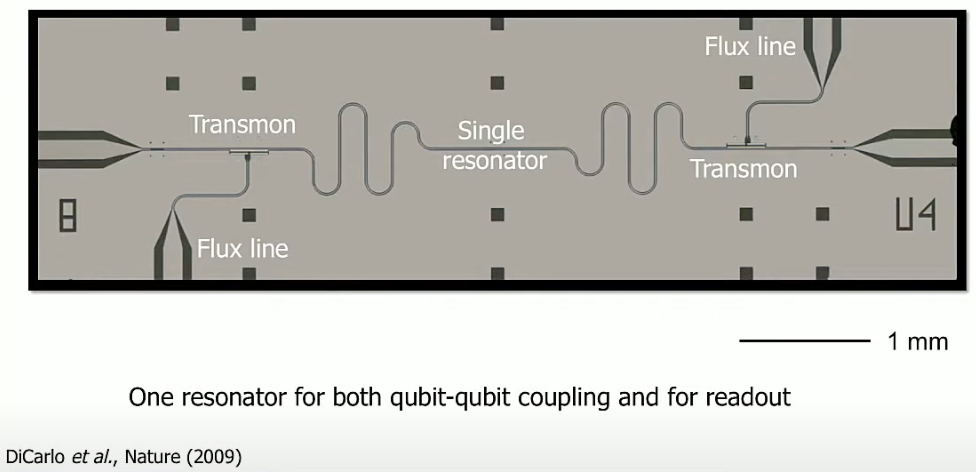
This image shows two qubits (transmons) coupled through a resonator (indirect coupling). Note the text below indicating that the resonator also functions as a coupler between the two qubits.

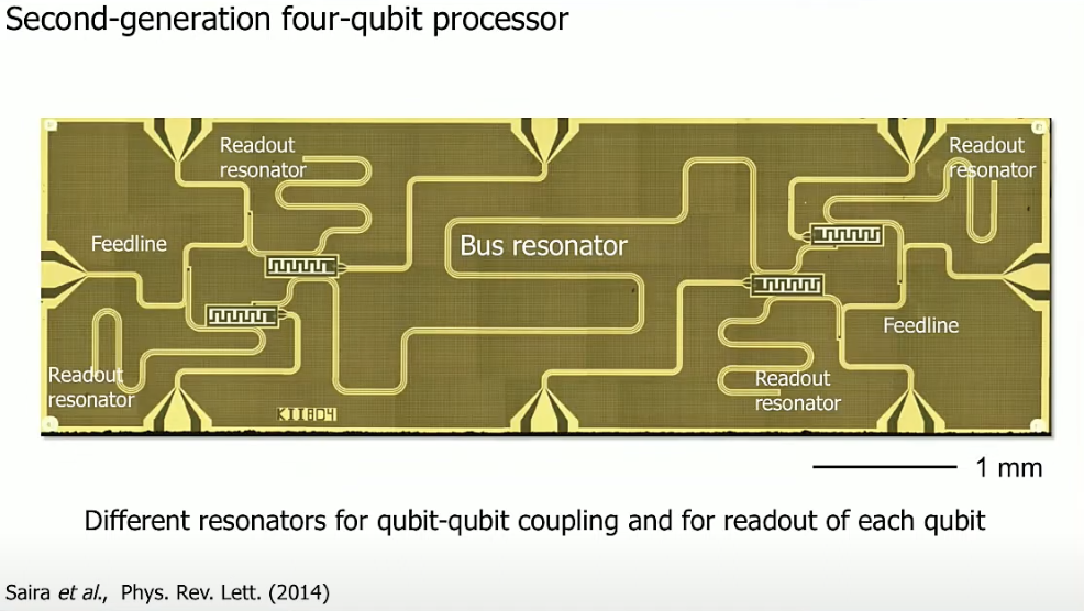
This image shows four qubits connected via a bus resonator. Each qubit is directly connected to flux lines, and there are readout feedlines on the top-\mathcal{L}eft and bottom-right. Each feedline is connected to two readout resonators, coupling with two qubits simultaneously.

doi.org/10.1038/nature13171
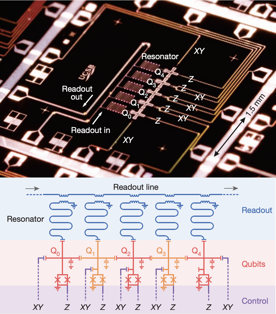
This is a schematic of a 5-qubit layout. Here, Z represents flux lines, and XY represents drive lines. The five qubits are directly coupled via capacitors. Each qubit has its own readout resonator, which merges (inductively coupled) into the readout line.

Towards Multi-Qubit Modules

https://arxiv.org/pdf/1612.08208
To achieve quantum computation, many qubits must be operated simultaneously. Due to error correction requirements, additional qubits are needed for this purpose. Above is an experimental 17-qubit quantum chip, arranged in a surface code configuration for quantum error correction. The qubits are shown in pink and red circles as data qubits, and light blue and green as check qubits. Each qubit connects to seven lines (nicknamed Starmon), including four for qubit coupling, one flux line, one drive line, and one readout resonator. The readout resonators are merged into three feedlines.

Introduction to Quantum LC Circuits

In quantum physics, a harmonic oscillator, after quantization, produces discrete energy levels, which form the foundational concept of qubits in quantum computing. Qubits rely on components exhibiting quantum effects. By using superconductors as quantum materials combined with the concept of LC oscillatory circuits, superconducting qubits can be manufactured. This section will first discuss the quantization process of LC circuits.

A basic \(LC\) oscillatory circuit consists of an inductor \(L\) and a capacitor \(C\). Defining the charge stored in the capacitor as \(Q\), the rate of change of \(Q\) (\(\dot{Q}\)) represents the current in the circuit. The energy stored in the capacitor and inductor can be expressed as: \[ E_C = \frac{Q^2}{2C}, \quad E_L = \frac{L\dot{Q}^2}{2}. \] We can interpret \(E_L\) as the kinetic energy term \(T\) and \(E_C\) as the potential energy term \(U\), thereby defining the Lagrangian \(\mathcal{L}\): \[ \mathcal{L}(\dot{Q}, Q) = T - U = \frac{L\dot{Q}^2}{2} - \frac{Q^2}{2C}. \]

According to the Euler-\mathcal{L}agrange equation: \[ \frac{d}{dt} \frac{\partial \mathcal{L}}{\partial \dot{Q}} - \frac{\partial \mathcal{L}}{\partial Q} = 0, \] we obtain: \[ L\ddot{Q} + \frac{Q}{C} = 0 \implies \ddot{Q} + \frac{Q}{LC} = 0, \] which describes simple harmonic motion with a frequency of \(\omega = \frac{1}{\sqrt{LC}}\).

Canonical Quantization of LC Circuits

Canonical quantization is a method for introducing quantum structure into classical systems by replacing the Poisson structure of the Hamiltonian with commutator relations. In the previous section, we derived the Lagrangian. Now, the Hamiltonian can be obtained via the Legendre transform.

The canonical momentum \(\Phi_\#\) is defined as: \[ \Phi_\# \equiv \frac{\partial \mathcal{L}}{\partial \dot{Q}} = \mathcal{L}\dot{Q} \leftrightarrow \dot{Q} = \frac{\Phi_\#}{L}. \] Here, \(\Phi_\#\) has the same unit as magnetic flux and can be interpreted as the flux inside the inductor. The Hamiltonian \(H(\Phi_\#, Q)\) is defined as: \[ \mathcal{H} \equiv \Phi_\# \dot{Q} - \mathcal{L} = \frac{\Phi_\#^2}{2L} + \frac{Q^2}{2C}. \]

In a quantum system, canonical coordinates \(q\) and canonical momentum \(p\) satisfy the commutator relation: \[ [x, p] = i\hbar. \] For the parameters in this paper, the quantization condition becomes: \[ [Q, \Phi_\#] = i\hbar. \]

For this discussion, we use \(\Phi_\#\) as the notation because it aligns with the traditional literature where the roles of \(\Phi_\#\) and \(Q\) in the Hamiltonian are symmetric. By convention, this paper reverses the traditional approach and treats flux as the generalized coordinate, denoted as \(\Phi\), while \(Q\) becomes the generalized momentum. Consequently, the quantization condition becomes: \[ [\Phi, Q] = i\hbar, \] with a sign difference: \[ \Phi = -\Phi_\#. \] This sign can be further explained by the antisymmetric nature of the Lagrangian.

To proceed, we introduce new variables \(a\) and \(a^\dagger\): \[ a = \sqrt{\frac{1}{2\hbar} \sqrt{\frac{L}{C}}} \left( Q + i\sqrt{\frac{C}{L}} \Phi_\# \right), \quad a^\dagger = \sqrt{\frac{1}{2\hbar} \sqrt{\frac{L}{C}}} \left( Q - i\sqrt{\frac{C}{L}} \Phi_\# \right). \] Conversely, these can be expressed as: \[ Q = \sqrt{\frac{\hbar}{2} \sqrt{\frac{C}{L}}} (a^\dagger + a), \quad \Phi_\# = i\sqrt{\frac{\hbar}{2} \sqrt{\frac{L}{C}}} (a^\dagger - a). \]

It can be shown that \([a, a^\dagger] = 1\): \[ [a, a^\dagger] = aa^\dagger - a^\dagger a = \frac{1}{2\hbar} \sqrt{\frac{L}{C}} \left[ Q, \Phi_\# \right] = 1. \] The Hamiltonian \(H(\Phi_\#, Q)\) can be rewritten as: \[ \mathcal{H} = \frac{\Phi_\#^2}{2L} + \frac{Q^2}{2C} = \frac{\hbar \omega}{4} \left[ - (a^\dagger - a)^2 + (a^\dagger + a)^2 \right], \] where \(\omega = \frac{1}{\sqrt{LC}}\). Expanding yields: \[ \mathcal{H} = \frac{\hbar \omega}{2} \left[ a^\dagger a + a^\dagger a + 1 \right] = \hbar \omega \left[ a^\dagger a + \frac{1}{2} \right]. \]

Finally, the quantized Hamiltonian is obtained, with each energy level separated by \(\hbar \omega\).

Interchange Between Kinetic and Potential Energy Terms

In practice, to correctly perform quantization via the commutator relation, it is essential to strictly define the correspondence between \(x, p\); otherwise, sign discrepancies might arise. Continuing from the previous section, we know: \[ \dot{\Phi}_\# = \frac{d}{dt} \frac{\partial \mathcal{L}}{\partial \dot{Q}} = \frac{\partial \mathcal{L}}{\partial Q} = -\frac{Q}{C} \implies Q = -C\dot{\Phi}_\#. \] Now, we transform the Lagrangian \(L\) into momentum space.

Define a new Lagrangian \(\bar{\mathcal{L}}\) as: \[ \bar{\mathcal{L}} \equiv \mathcal{L} - \frac{d}{dt} (\Phi_\# Q) = \mathcal{L} - \dot{\Phi}_\# Q - \Phi_\# \dot{Q}, \] Expanding this yields: \[ \bar{\mathcal{L}} = \frac{L\dot{Q}^2}{2} - \frac{Q^2}{2C} - \dot{\Phi}_\# Q - \Phi_\# \dot{Q} = \frac{\Phi_\#^2}{2L} - \frac{C\dot{\Phi}_\#^2}{2} + C\dot{\Phi}_\#^2 - \frac{\Phi_\#^2}{L}, \] Simplifying to: \[ \bar{\mathcal{L}} = \frac{C\dot{\Phi}_\#^2}{2} - \frac{\Phi_\#^2}{2L}. \]

Note that at this point \(\mathcal{L}(Q, \dot{Q}) \to \bar{\mathcal{L}}(\Phi_\#, \dot{\Phi}_\#)\), and the roles of kinetic and potential energy are interchanged. Additionally, \(\bar{\mathcal{L}} = -\mathcal{L}\), corresponding to the antisymmetry of the Lagrangian. To absorb this antisymmetry, we define a new variable: \[ \Phi = -\Phi_\#. \] This ensures: \[ \bar{\mathcal{L}}(\dot{\Phi}, \Phi) = \frac{C\dot{\Phi}^2}{2} - \frac{\Phi^2}{2L}. \]

The corresponding canonical momentum \(\Pi\) (related to \(Q\) based on previous results): \[ \Pi \equiv \frac{\partial \bar{\mathcal{L}}}{\partial \dot{\Phi}} = C\dot{\Phi} = -C\dot{\Phi}_\# = Q \implies \dot{\Phi} = \frac{\Pi}{C} = \frac{Q}{C}. \]

The Hamiltonian \(\bar{\mathcal{H}} \) is defined as: \[ \bar{\mathcal{H}} = \Pi\dot{\Phi} - \bar{\mathcal{L}} = \frac{\Pi^2}{C} - \frac{\Pi^2}{2C} + \frac{\Phi^2}{2L} = \frac{\Pi^2}{2C} + \frac{\Phi^2}{2L}, \] which matches the previous \(\mathcal{H}\) exactly. The quantization condition becomes: \[ [\Phi, \Pi] = [\Phi, Q] = i\hbar, \] identical to the traditional condition.

Define new variables \(a\) and \(a^\dagger\): \[ a = \sqrt{\frac{1}{2\hbar} \sqrt{\frac{L}{C}}} \left( \sqrt{\frac{C}{L}} \Phi + iQ \right), \quad a^\dagger = \sqrt{\frac{1}{2\hbar} \sqrt{\frac{L}{C}}} \left( \sqrt{\frac{C}{L}} \Phi - iQ \right). \] Conversely: \[ \Phi = \sqrt{\frac{\hbar}{2} \sqrt{\frac{L}{C}}} (a^\dagger + a), \quad Q = i\sqrt{\frac{\hbar}{2} \sqrt{\frac{C}{L}}} (a^\dagger - a). \]

It is easy to verify \([a, a^\dagger] = 1\): \[ [a, a^\dagger] = aa^\dagger - a^\dagger a = \frac{1}{2\hbar} \sqrt{\frac{L}{C}} \left[ \Phi, Q \right] = 1. \] The Hamiltonian \(H(\Phi, Q)\) can be rewritten as: \[ \mathcal{H} = \frac{\Phi^2}{2L} + \frac{Q^2}{2C} = \frac{\hbar}{4\sqrt{LC}} \left[ (a^\dagger + a)^2 - (a^\dagger - a)^2 \right]. \] Given \(\omega = \frac{1}{\sqrt{LC}}\), expanding this yields: \[ \mathcal{H} = \frac{\hbar \omega}{4} \left[ (a^\dagger + a)^2 - (a^\dagger - a)^2 \right] = \hbar \omega \left[ a^\dagger a + \frac{1}{2} \right]. \]

Finally, we once again obtain the quantized Hamiltonian, where the difference between each energy level is \(\hbar \omega\).

Formalizing the Interchange of Kinetic and Potential Energy in the Lagrangian

Starting from \(L(\dot{Q}, Q)\), based on the antisymmetry between the kinetic and potential energy in the Lagrangian, we manually introduce a negative sign when defining the canonical momentum \(\Phi\) corresponding to \(\dot{Q}\) to absorb this antisymmetry (otherwise, the resulting Hamiltonian would be negative): \[ \Phi \equiv -\frac{\partial \mathcal{L}}{\partial \dot{Q}} \implies \dot{\Phi} = -\frac{\partial \mathcal{L}}{\partial Q}. \] Next, we switch the Lagrangian to the \((\dot{\Phi}, \Phi)\) space, i.e., the momentum-space Lagrangian \(\bar{\mathcal{L}}\): \[ \bar{\mathcal{L}} \equiv \mathcal{L} + \frac{d}{dt} (\Phi Q) = \mathcal{L} + \dot{\Phi} Q + \Phi \dot{Q}. \]

Using differential techniques, we can prove that \(\bar{\mathcal{L}} = \bar{\mathcal{L}}(\dot{\Phi}, \Phi)\) is indeed a function of \((\dot{\Phi}, \Phi)\) space: \[ d\bar{\mathcal{L}} = d\mathcal{L} + d(\dot{\Phi} Q) + d(\Phi \dot{Q}) = \frac{\partial \mathcal{L}}{\partial \dot{Q}} d\dot{Q} + \frac{\partial \mathcal{L}}{\partial Q} dQ + Qd\dot{\Phi} + \dot{\Phi}dQ + \dot{Q}d\Phi + \Phi d\dot{Q}. \] Expanding further, since \(-\Phi = \frac{\partial \mathcal{L}}{\partial \dot{Q}}\), we have: \[ d\bar{\mathcal{L}} = -\Phi d\dot{Q} - \dot{\Phi} dQ + Q d\dot{\Phi} + \dot{\Phi} dQ + \dot{Q} d\Phi + \Phi d\dot{Q} = Q d\dot{\Phi} + \dot{Q} d\Phi. \]

The corresponding canonical momentum \(\Pi\) for \(\dot{\Phi}\) is: \[ \Pi = \frac{\partial \bar{\mathcal{L}}}{\partial \dot{\Phi}} = Q, \] which is the same as the original \(Q\). The corresponding Hamiltonian \(\bar{\mathcal{H}} \) is defined as: \[ \bar{\mathcal{H}} = \Pi \dot{\Phi} - \bar{\mathcal{L}} = Q\dot{\Phi} - \mathcal{L} - \dot{\Phi} Q - \Phi \dot{Q} = -\mathcal{L} - \Phi \dot{Q}. \] The final form is: \[ \bar{\mathcal{H}} (Q, \Phi) = -\mathcal{L} - \Phi \dot{Q}. \]

This allows us to simplify subsequent derivations by following these steps:

Write down \(L(\dot{Q}, Q)\).
Define \(\Phi \equiv -\frac{\partial \mathcal{L}}{\partial \dot{Q}}\) and establish the relationship between \(\dot{Q}\) and \(\Phi\).
Directly calculate the corresponding Hamiltonian: \[ \bar{\mathcal{H}} (Q, \Phi) = -\mathcal{L} - \Phi \dot{Q}, \] substituting \(\dot{Q}\) from the previous relationship.
Quantization condition: \[ [Q, \Phi] = i\hbar. \]

This eliminates the need for the cumbersome transformation \(L(\dot{Q}, Q) \to \bar{\mathcal{L}}(\dot{\Phi}, \Phi) \to \bar{\mathcal{H}} (Q, \Phi)\). Especially when introducing external coupling terms (e.g., in deriving how to drive and read quantum bits, external signals interacting with quantum bits, or coupling between two quantum bits), following the traditional approach would lead to extremely complex intermediate calculations, similar to the momentum shift \(p \to p - eA\) in an electromagnetic field.

Note: \[ \bar{\mathcal{H}} (Q, \Phi) = -\mathcal{L} - \Phi \dot{Q} = -\mathcal{L} + \frac{\partial \mathcal{L}}{\partial \dot{Q}} \dot{Q} = H(\Phi, Q). \] \(H(\Phi, Q)\) is the familiar Hamiltonian in classical mechanics. Moreover, \(\bar{\mathcal{H}} = H\) reaffirms the symmetry between kinetic and potential energy in the Hamiltonian.

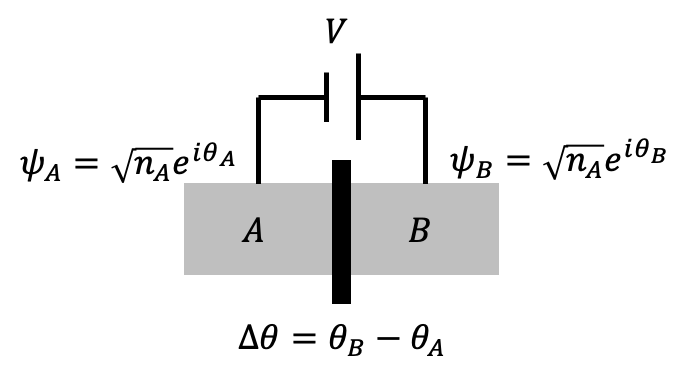
Nonlinear Inductance of Josephson Junctions

A Josephson junction can be described with its intrinsic properties represented by \(H_0\). When a voltage \(V\) is applied across the junction, the interaction between the superconducting wavefunctions is represented by \(K\). The equation of motion is given as: \[ i\hbar \frac{\partial}{\partial t} \begin{pmatrix} \sqrt{n_A} e^{i\theta_A} \\ \sqrt{n_B} e^{i\theta_B} \end{pmatrix} = \begin{pmatrix} H_0 - \frac{qV}{2} & K \\ K & H_0 + \frac{qV}{2} \end{pmatrix} \begin{pmatrix} \sqrt{n_A} e^{i\theta_A} \\ \sqrt{n_B} e^{i\theta_B} \end{pmatrix}. \] When \(q = -2e\) (Cooper pairs), the equation becomes: \[ i\hbar \frac{\partial}{\partial t} \begin{pmatrix} \sqrt{n_A} e^{i\theta_A} \\ \sqrt{n_B} e^{i\theta_B} \end{pmatrix} = \begin{pmatrix} H_0 + eV & K \\ K & H_0 - eV \end{pmatrix} \begin{pmatrix} \sqrt{n_A} e^{i\theta_A} \\ \sqrt{n_B} e^{i\theta_B} \end{pmatrix}. \]

Derivation for \(\theta_A, n_A\)

The first equation is: \[ i\hbar \frac{\partial}{\partial t} (\sqrt{n_A} e^{i\theta_A}) = \frac{i}{2} \frac{e^{i\theta_A}}{\sqrt{n_A}} \frac{\partial n_A}{\partial t} - \sqrt{n_A} e^{i\theta_A} \frac{\partial \theta_A}{\partial t} = (H_0 + eV) \sqrt{n_A} e^{i\theta_A} + K\sqrt{n_B} e^{i\theta_B}. \] Separating the real and imaginary parts gives: \[ \frac{i}{2}\hbar \frac{\partial n_A}{\partial t} - n_A \hbar \frac{\partial \theta_A}{\partial t} = (H_0 + eV)n_A + K\sqrt{n_A n_B} e^{i(\theta_B - \theta_A)}. \] Its conjugate equation is: \[ -\frac{i}{2}\hbar \frac{\partial n_A}{\partial t} - n_A \hbar \frac{\partial \theta_A}{\partial t} = (H_0 + eV)n_A + K\sqrt{n_A n_B} e^{-i(\theta_B - \theta_A)}. \]

Adding the two equations gives: \[ -2n_A \hbar \frac{\partial \theta_A}{\partial t} = 2(H_0 + eV)n_A + 2K\sqrt{n_A n_B} \cos(\theta_B - \theta_A), \] yielding the equation for \(\theta_A\): \[ \hbar \frac{\partial \theta_A}{\partial t} = -(H_0 + eV) - K\sqrt{\frac{n_B}{n_A}} \cos(\theta_B - \theta_A). \]
Subtracting the two equations gives: \[ i\hbar \frac{\partial n_A}{\partial t} = 2iK\sqrt{n_A n_B} \sin(\theta_B - \theta_A), \] which simplifies to: \[ \hbar \frac{\partial n_A}{\partial t} = 2K\sqrt{n_A n_B} \sin(\theta_B - \theta_A). \]

Derivation for \(\theta_B, n_B\)

The second equation is: \[ i\hbar \frac{\partial}{\partial t} (\sqrt{n_B} e^{i\theta_B}) = \frac{i}{2} \frac{e^{i\theta_B}}{\sqrt{n_B}} \frac{\partial n_B}{\partial t} - \sqrt{n_B} e^{i\theta_B} \frac{\partial \theta_B}{\partial t} = K\sqrt{n_A} e^{i\theta_A} + (H_0 - eV)\sqrt{n_B} e^{i\theta_B}. \] Separating this gives: \[ \frac{i}{2}\hbar \frac{\partial n_B}{\partial t} - n_B \hbar \frac{\partial \theta_B}{\partial t} = K\sqrt{n_A n_B} e^{-i(\theta_B - \theta_A)} + (H_0 - eV)n_B. \] Its conjugate equation is: \[ -\frac{i}{2}\hbar \frac{\partial n_B}{\partial t} - n_B \hbar \frac{\partial \theta_B}{\partial t} = K\sqrt{n_A n_B} e^{i(\theta_B - \theta_A)} + (H_0 - eV)n_B. \]

Adding the two equations gives: \[ -2n_B \hbar \frac{\partial \theta_B}{\partial t} = 2K\sqrt{n_A n_B} \cos(\theta_B - \theta_A) + 2(H_0 - eV)n_B, \] which simplifies to: \[ \hbar \frac{\partial \theta_B}{\partial t} = -(H_0 - eV) - K\sqrt{\frac{n_A}{n_B}} \cos(\theta_B - \theta_A). \]
Subtracting the two equations gives: \[ i\hbar \frac{\partial n_B}{\partial t} = -2iK\sqrt{n_A n_B} \sin(\theta_B - \theta_A), \] which simplifies to: \[ \hbar \frac{\partial n_B}{\partial t} = -2K\sqrt{n_A n_B} \sin(\theta_B - \theta_A). \]

Combining these results:

For \(\theta_A\): \[ \hbar \frac{\partial \theta_A}{\partial t} = -(H_0 + eV) - K\sqrt{\frac{n_B}{n_A}} \cos(\theta_B - \theta_A). \]
For \(\theta_B\): \[ \hbar \frac{\partial \theta_B}{\partial t} = -(H_0 - eV) - K\sqrt{\frac{n_A}{n_B}} \cos(\theta_B - \theta_A). \]
For \(n_A\): \[ \hbar \frac{\partial n_A}{\partial t} = 2K\sqrt{n_A n_B} \sin(\theta_B - \theta_A). \]
For \(n_B\): \[ \hbar \frac{\partial n_B}{\partial t} = -2K\sqrt{n_A n_B} \sin(\theta_B - \theta_A). \]

Defining the phase difference \(\Delta \theta = \theta_B - \theta_A\) and combining the first two equations, we find: \[ \hbar \frac{\partial \Delta \theta}{\partial t} = 2eV + \frac{K}{\hbar} \left( \frac{n_B - n_A}{\sqrt{n_A n_B}} \right) \cos\Delta \theta. \] Combining the last two equations and defining the current \(I\) as: \[ -\frac{\partial n_A}{\partial t} = \frac{\partial n_B}{\partial t} \equiv \frac{I}{-2e}, \] we obtain: \[ I = \frac{4eK}{\hbar} \sqrt{n_A n_B} \sin\Delta \theta \equiv I_c \sin\Delta \theta, \] where \(I_c\) is the critical current of the Josephson junction.

The nonlinear inductance of the Josephson junction is defined as: \[ L_J(\Delta \theta) = \left(\frac{2e}{\hbar I_c \cos\Delta \theta}\right). \] The energy stored in the inductance is: \[ E = \int IV dt = \int I_0 \sin\Delta \theta \cdot \frac{\hbar}{q} \frac{\partial \Delta \theta}{\partial t} dt = -\frac{I_0 \hbar}{2e} \cos\Delta \theta \equiv -\frac{I_0 \Phi_0}{2\pi} \cos\Delta \theta, \] where the flux quantum is \(\Phi_0 = \frac{2\pi\hbar}{2e}\), and: \[ E_J = \frac{I_0 \Phi_0}{2\pi}. \]

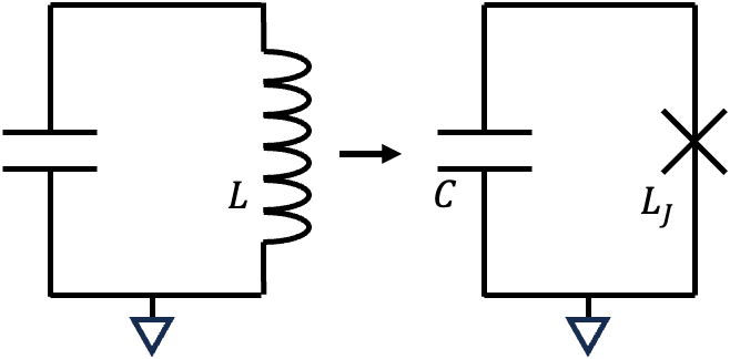
▲ Transforming a linear \(LC\) circuit into a nonlinear \(LC\) circuit by incorporating the nonlinear inductance of Josephson junctions. \(L_J\) represents the inductance of the Josephson junction.

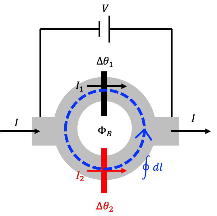
Nonlinear Inductance of a Double Josephson Junction (SQUID)

Two Josephson junctions, \(J_1\) and \(J_2\), are connected to form a closed loop, with a magnetic flux \(\Phi_B\) and voltage \(V\) applied. According to the previous section, the integral of the superconducting wavefunction phase around the loop must satisfy: \[ \oint \nabla \theta(r) \cdot d\vec{l} - \frac{q}{\hbar} \Phi_B = 2\pi N. \] Since discontinuities at the junctions contribute \(\Delta\theta_1\) and \(\Delta\theta_2\), and with \(q = -2e\), this becomes: \[ \Delta\theta_2 - \Delta\theta_1 + 2\pi \frac{\Phi_B}{\Phi_0} = 2\pi N, \] leading to: \[ \Delta\theta_2 = \Delta\theta_1 - 2\pi \frac{\Phi_B}{\Phi_0} + 2\pi N. \]

When the entire SQUID loop carries a current \(I = I_1 + I_2\), and using the Josephson current relation from the previous section (assuming a symmetric SQUID with both junctions having the same \(I_c\)), we compute: \[ I = I_1 + I_2 = I_0 (\sin\Delta\theta_1 + \sin\Delta\theta_2). \] Substituting \(\Delta\theta_2\): \[ I = I_0 \left[\sin\Delta\theta_1 + \sin\left(\Delta\theta_1 - 2\pi \frac{\Phi_B}{\Phi_0} + 2\pi N\right)\right]. \] Simplifying (noting that \(N\) is an integer and does not affect the sine function): \[ I = I_0 \left[\sin\Delta\theta_1 + \sin\left(\Delta\theta_1 - 2\pi \frac{\Phi_B}{\Phi_0}\right)\right]. \] Using trigonometric identities: \[ I = I_0 \left[2 \sin\left(\frac{\Delta\theta_1 + \Delta\theta_1 - 2\pi \frac{\Phi_B}{\Phi_0}}{2}\right) \cos\left(\frac{\Delta\theta_1 - \Delta\theta_1 + 2\pi \frac{\Phi_B}{\Phi_0}}{2}\right)\right]. \] This simplifies to: \[ I = 2I_0 \cos\left(\frac{\Phi_B}{\Phi_0} \pi\right) \sin\left(\Delta\theta_1 - \frac{\Phi_B}{\Phi_0} \pi\right). \]

From the previous section, Josephson junctions exhibit inductive properties. Similarly, we can discuss the inductance of the SQUID. Differentiating the current with respect to time gives: \[ \dot{I} = 2I_0 \cos\left(\frac{\Phi_B}{\Phi_0} \pi\right) \cos\left(\Delta\theta_1 - \frac{\Phi_B}{\Phi_0} \pi\right) \dot{\Delta\theta_1}. \] The relationship between \(\dot{\Delta\theta_1}\) and the voltage \(V\) is: \[ V = \frac{\hbar}{2e} \dot{\Delta\theta_1} = \frac{\Phi_0}{2\pi} \dot{\Delta\theta_1}. \] Substituting this, we find the inductance: \[ L_{\text{SQUID}}(\Delta\theta_1, \Phi_B) = \left[\frac{2\pi}{\Phi_0} \cdot 2I_0 \cos\left(\frac{\Phi_B}{\Phi_0} \pi\right) \cos\left(\Delta\theta_1 - \frac{\Phi_B}{\Phi_0} \pi\right)\right]. \]

Notice that the value of \(L_{\text{SQUID}}\) is influenced by the external magnetic flux \(\Phi_B\), which is key for tuning the frequency in Tunable Transmons. Defining the variable \(\Phi\): \[ \Phi \equiv \frac{\Delta\theta_1}{\pi} \Phi_0 - \Phi_B = \frac{\Phi_0}{\pi} \left(\Delta\theta_1 - \frac{\Phi_B}{\Phi_0} \pi\right), \] with: \[ \dot{\Phi} = \frac{\Phi_0}{\pi} \dot{\Delta\theta_1}. \] The voltage \(V\) and current \(I\) are: \[ V = \frac{1}{2} \dot{\Phi}, \quad I = 2I_0 \cos\left(\frac{\Phi_B}{\Phi_0} \pi\right) \sin\left(\frac{\Phi}{\Phi_0} \pi\right). \]

For a fixed external flux \(\Phi_B\), the energy stored in a SQUID is: \[ E = \int IV \, dt = \int \left[2I_0 \cos\left(\frac{\Phi_B}{\Phi_0} \pi\right) \sin\left(\frac{\Phi}{\Phi_0} \pi\right) \cdot \frac{1}{2} \dot{\Phi}\right] dt. \] Simplifying gives: \[ E = I_0 \cos\left(\frac{\Phi_B}{\Phi_0} \pi\right) \int \sin\left(\frac{\Phi}{\Phi_0} \pi\right) d\Phi. \] Resulting in: \[ E = -\frac{I_0 \Phi_0}{\pi} \cos\left(\frac{\Phi_B}{\Phi_0} \pi\right) \cos\left(\frac{\pi}{\Phi_0} \Phi\right). \]

▲An \(LC\) circuit with tunable inductance formed by two Josephson junctions.

Properties of the Transmon

Ref: DOI:10.48550/arXiv.2203.04164

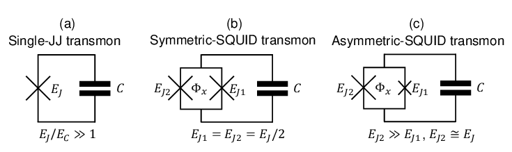
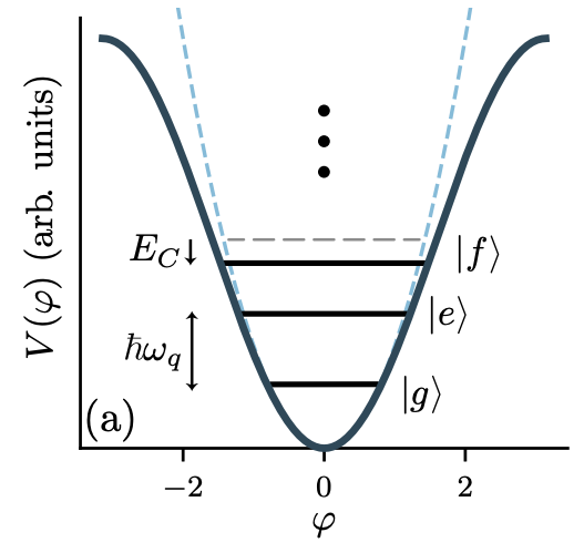
As mentioned previously, Josephson junctions exhibit inductive properties, and the Transmon is a variant of an LC circuit where the inductance is replaced by a Josephson junction. This section directly discusses the Tunable Transmon, where a SQUID is used as the inductance. In practice, due to material inhomogeneity, different Transmons may have different properties. However, by using a Tunable Transmon, the qubit properties can be made consistent by fine-tuning the magnetic flux \(\Phi_B\). Additionally, as we discussed earlier when quantizing the LC circuit, \([ \Phi, Q ] = i\hbar\) are conjugate variables. Using the derivation for the SQUID, we can naturally relate the magnetic flux \(\Phi\) to the phase difference \(\Delta\theta\), i.e.: \[ \Phi \equiv \frac{\Delta\theta_1}{\pi} \Phi_0 - \Phi_B. \]

Now, we write down the Hamiltonian: \[ \mathcal{H} = \frac{Q^2}{2C} + \frac{\Phi_\#^2}{2L} = \frac{Q^2}{2C} + \frac{(I_0 \pi)}{2\Phi_0} \cos\left(\frac{\Phi_B}{\Phi_0} \pi\right) \Phi^2 - \frac{I_0}{24} \left(\frac{\pi}{\Phi_0}\right)^3 \cos\left(\frac{\Phi_B}{\Phi_0} \pi\right) \Phi^4 + \cdots \] \[ = \frac{Q^2}{2C} + \frac{\Phi^2}{2L} - \frac{1}{24L} \left(\frac{\pi}{\Phi_0}\right)^2 \Phi^4 + \cdots \] where: \[ L = \left(\frac{I_0 \pi}{\Phi_0} \cos\left(\frac{\Phi_B}{\Phi_0} \pi\right)\right)^{-1}. \]

Next, we discuss how the nonlinearity affects the energy levels. From earlier, we selected new variables \( a \), \( a^\dagger \): \[ a = \sqrt{\frac{1}{2\hbar} \sqrt{ \frac{L}{C}}} \left(\sqrt{\frac{C}{L}} \Phi + iQ\right), \quad a^\dagger = \sqrt{\frac{1}{2\hbar} \sqrt{ \frac{L}{C}}} \left(\sqrt{\frac{C}{L}} \Phi - iQ\right). \] Conversely: \[ \Phi = \sqrt{\frac{\hbar}{2 }\sqrt{ \frac{L}{C}}} (a^\dagger + a), \quad Q = i\sqrt{\frac{\hbar}{2} \sqrt{ \frac{C}{L}}} (a^\dagger - a). \]

Expanding the Hamiltonian: \[ \mathcal{H} = \frac{\hbar}{\sqrt{LC}} \left[a^\dagger a + \frac{1}{2}\right] - \frac{1}{24L} \left(\frac{\pi}{\Phi_0}\right)^2 \left[i \sqrt{\frac{\hbar}{2\sqrt{L/C}}} (a^\dagger + a)\right]^4. \] Simplifying: \[ \mathcal{H} = \frac{\hbar}{\sqrt{LC}} \left[a^\dagger a + \frac{1}{2}\right] - \frac{\hbar^2}{96C} \left(\frac{\pi}{\Phi_0}\right)^2 (a^\dagger + a)^4. \] This expression contains both linear and nonlinear terms, where the linear terms describe the energy levels of a quantum harmonic oscillator, and the nonlinear terms arise from the Josephson junction's correction to the energy levels.

Using perturbation theory, when \( \mathcal{H} = H_0 + \Delta H \), and \( |E_0^m\rangle \to |E^m\rangle \), \( E_0^m \to E^m = E_0^m + \delta E^m \), we know the energy correction \( \delta E^m \) to the energy level \( E_0^m \) is:

\[ \delta E^m = \langle E_0^m | \Delta H | E_0^m \rangle = \langle E_0^m | \left[-\frac{\hbar^2}{96C} \left(\frac{\pi}{\Phi_0}\right)^2 (a^\dagger + a)^4\right] | E_0^m \rangle. \]

Expanding this:

\[ \langle E_0^m | (a^\dagger + a)^4 | E_0^m \rangle = \langle E_0^m | (aa + aa^\dagger + a^\dagger a + a^\dagger a^\dagger)^2 | E_0^m \rangle. \]

Expanding further:

\[ \langle E_0^m | aa(aa + aa^\dagger + a^\dagger a + a^\dagger a^\dagger) + aa^\dagger(aa + aa^\dagger + a^\dagger a + a^\dagger a^\dagger) + a^\dagger a(aa + aa^\dagger + a^\dagger a + a^\dagger a^\dagger) + a^\dagger a^\dagger(aa + aa^\dagger + a^\dagger a + a^\dagger a^\dagger) | E_0^m \rangle. \]

Taking the expectation value, we only keep terms where \( a \) and \( a^\dagger \) appear with equal powers, resulting in:

\[ \langle E_0^m | aaa^\dagger a^\dagger + aa^\dagger aa^\dagger + aa^\dagger a^\dagger a + a^\dagger aaa^\dagger + a^\dagger aa^\dagger a + a^\dagger a^\dagger aa | E_0^m \rangle. \]

Simplifying further:

\[ \langle E_0^m | a(a^\dagger a + 1)a^\dagger + aa^\dagger aa^\dagger + (a^\dagger a + 1)a^\dagger a + a^\dagger a(a^\dagger a + 1) + a^\dagger aa^\dagger a + a^\dagger (aa^\dagger - 1)a | E_0^m \rangle. \]

Further simplifying:

\[ \langle E_0^m | aa^\dagger aa^\dagger + aa^\dagger + aa^\dagger aa^\dagger + a^\dagger aa^\dagger a + a^\dagger a + a^\dagger aa^\dagger a + a^\dagger a + a^\dagger aa^\dagger a + a^\dagger aa^\dagger a - a^\dagger a | E_0^m \rangle. \]

After further simplification:

\[ \langle E_0^m | 2aa^\dagger aa^\dagger + aa^\dagger + 4a^\dagger aa^\dagger a + a^\dagger a | E_0^m \rangle. \]

This simplifies to:

\[ \langle E_0^m | 2(a^\dagger a + 1)(a^\dagger a + 1) + (a^\dagger a + 1) + 4a^\dagger aa^\dagger a + a^\dagger a | E_0^m \rangle. \]

Finally, the energy level correction is:

\[ \langle E_0^m | 6a^\dagger aa^\dagger a + 6a^\dagger a + 3 | E_0^m \rangle = 6m^2 + 6m + 3. \]

The energy difference between levels \(m\) and \(m-1\) is:

\[ \Delta E^m_{m-1} = \frac{\hbar}{\sqrt{LC}} - \frac{\hbar^2}{96C} \left(\frac{\pi}{\Phi_0}\right)^2 \left\{6[m^2 - (m-1)^2] + 6\right\}. \]

\[ = \frac{\hbar}{\sqrt{LC}} - \frac{\hbar^2 \pi^2}{96C} \frac{e^2}{\pi^2 \hbar^2} \left[6(2m - 1) + 6\right]. \]

Finally, we get:

\[ \Delta E^m_{m-1} = \frac{\hbar}{\sqrt{LC}} - m\frac{e^2}{8C}. \]

Calculating \( \Delta E^{21} - \Delta E^{10} \):

\[ \Delta E^{21} - \Delta E^{10} = \left(\frac{\hbar}{\sqrt{LC}} - 2\frac{e^2}{8C}\right) - \left(\frac{\hbar}{\sqrt{LC}} - \frac{e^2}{8C}\right). \]

\[ = -\frac{e^2}{8C} \equiv -E_C. \]

\( E_C \) represents the nonlinear effect.

Ref: DOI:10.1103/RevModPhys.93.025005

Computational Science and Two-Level Systems (TLS)

The fundamental principle behind modern computers relies on bits for storing information and logic gates for computation. Information is encoded in binary as sequences of 0s and 1s. These bits are manipulated to store information. For example, to store the number 19, its binary representation is 10011. When stored in an 8-bit memory, the state becomes:

\[ \ket{bit_1} \ket{bit_2} \ket{bit_3} \ket{bit_4} \ket{bit_5} \ket{bit_6} \ket{bit_7} \ket{bit_8} \] changing to: \[ \ket{0} \ket{0} \ket{0} \ket{1} \ket{0} \ket{0} \ket{1} \ket{1} \]

In a quantum harmonic oscillator, the different energy levels \( n \) can be connected using \( a^\dagger \) and \( a \):

\[ \ket{n+1} = \frac{a^\dagger}{\sqrt{n+1}} \ket{n}, \quad \ket{n-1} = \frac{a}{\sqrt{n}} \ket{n}, \quad \ket{n} = \frac{(a^\dagger)^n}{\sqrt{n!}} \ket{0} \]

In this case:

\[ a^\dagger = \begin{bmatrix} 0 & 1 & 0 & \cdots \\ 0 & 0 & \sqrt{2} & \cdots \\ 0 & 0 & 0 & \cdots \\ \vdots & \vdots & \vdots & \ddots \\ \end{bmatrix} \]

\[ a = \begin{bmatrix} 0 & 0 & 0 & \cdots \\ 1 & 0 & 0 & \cdots \\ 0 & \sqrt{2} & 0 & \cdots \\ \vdots & \vdots & \vdots & \ddots \\ \end{bmatrix} \]

This represents an infinite-dimensional quantum system. A superconducting qubit uses the Transmon's ground state \( \ket{0} \) (or \( \ket{g} \)) and the first excited state \( \ket{1} \) (or \( \ket{e} \)) as its computational basis. In the two-dimensional framework of quantum computation:

\[ a^\dagger \rightarrow \sigma^+ = \begin{bmatrix} 0 & 1 \\ 0 & 0 \\ \end{bmatrix}, \quad a \rightarrow \sigma^- = \begin{bmatrix} 0 & 0 \\ 1 & 0 \\ \end{bmatrix} \]

These lead to the following definitions:

\[ \sigma_x = \sigma^+ + \sigma^- = \begin{bmatrix} 0 & 1 \\ 1 & 0 \\ \end{bmatrix}, \quad \sigma_y = i \left(\sigma^+ - \sigma^- \right) = \begin{bmatrix} 0 & -i \\ i & 0 \\ \end{bmatrix}, \quad \sigma_z = \mathbb{I} - 2\sigma^+\sigma^- = \begin{bmatrix} 1 & 0 \\ 0 & -1 \\ \end{bmatrix} \]

These are the famous Pauli matrices. Here are some algebraic relations:

\[ \{\sigma^-, \sigma^+\} = \sigma^-\sigma^+ + \sigma^+\sigma^- = \mathbb{I} = \begin{bmatrix} 1 & 0 \\ 0 & 1 \\ \end{bmatrix}, \quad [\sigma^-, \sigma^+] = \sigma^-\sigma^+ - \sigma^+\sigma^- = \sigma_z = \begin{bmatrix} 1 & 0 \\ 0 & -1 \\ \end{bmatrix} \]

For \( i, j, k = x, y, z \):

\[ \sigma_i \sigma_j = \delta_{ij}\mathbb{I} + i\epsilon_{ijk}\sigma_k \]

The Pauli matrices are deeply connected to rotations in three-dimensional space. However, one might wonder: why does a two-level qubit system relate to three-dimensional rotations? This will be discussed in the next section on qubits and the Bloch sphere representation.

Driving an LC Circuit

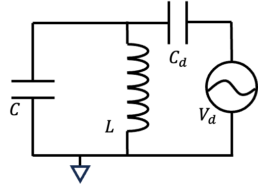
Now, let's discuss how to drive an LC circuit and a transmon qubit. By coupling the system to an external voltage source \( V_d \) through a coupling capacitor \( C_d \), the Lagrangian of the system is given by:

\[ \mathcal{L}_d(\dot{Q}, Q) = T - U = \frac{L\dot{Q}^2}{2} - \frac{Q^2}{2C} - \frac{Q_d^2}{2C_d} \]

The energy associated with the coupling capacitor \( C_d \) is:

\[ \frac{Q_d^2}{2C_d} = \frac{C_d (V - V_d)^2}{2} = \frac{C_d \left(\frac{Q}{C} - V_d\right)^2}{2} \] \[ = \frac{C_d Q^2}{2C^2} - \frac{C_d Q}{C}V_d + \frac{C_d V_d^2}{2} \]

Substituting the above expression into the Lagrangian and simplifying, we obtain:

\[ \mathcal{L}_d(\dot{Q}, Q) = \frac{L\dot{Q}^2}{2} - \frac{Q^2}{2C} - \frac{C_d}{C} \frac{Q^2}{2C} + \frac{C_d}{C} QV_d - \frac{C_d V_d^2}{2} \] \[ = \frac{L\dot{Q}^2}{2} - \frac{Q^2}{2C_\Sigma} + \frac{C_d}{C} QV_d - \frac{C_d V_d^2}{2} \]

Here, \( C_\Sigma = \frac{C^2}{C + C_d} \). We define the canonical momentum as:

\[ \Phi = -\frac{\partial \mathcal{L}_d}{\partial \dot{Q}} = -L\dot{Q} \quad \rightarrow \quad \dot{Q} = -\frac{\Phi}{L} \]

Next, we calculate the Hamiltonian:

\[ \bar{\mathcal{H}} _d = -\mathcal{L}_d - \Phi \dot{Q} = -\frac{L\dot{Q}^2}{2} + \frac{Q^2}{2C_\Sigma} - \frac{C_d}{C} QV_d + \frac{\Phi^2}{L} \] \[ = \frac{\Phi^2}{2L} + \frac{Q^2}{2C_\Sigma} - \frac{C_d}{C} QV_d \]

Detailed Derivation

Proceeding with canonical quantization:

\[ \begin{aligned} &a_d = \sqrt{\frac{1}{2\hbar} \sqrt{\frac{L}{C_\Sigma}}} \left(\sqrt{\frac{C_\Sigma}{L}} \Phi + iQ\right) \\ &a_d^\dagger = \sqrt{\frac{1}{2\hbar} \sqrt{\frac{L}{C_\Sigma}}} \left(\sqrt{\frac{C_\Sigma}{L}} \Phi - iQ\right) \end{aligned} \quad \leftrightarrow \quad \begin{aligned} &\Phi_d = \sqrt{\frac{\hbar}{2} \sqrt{\frac{L}{C_\Sigma}}} (a_d^\dagger + a_d) \\ &Q_d = i\sqrt{\frac{\hbar}{2} \sqrt{\frac{C_\Sigma}{L}}} (a_d^\dagger - a_d) \end{aligned} \]

Substituting these expressions, we obtain:

\[ = \hbar \sqrt{\frac{1}{LC_\Sigma}} \left( a_d^\dagger a_d + \frac{1}{2} \right) - \frac{C_d}{C} \sqrt{\frac{\hbar}{2 C_\Sigma \sqrt{LC_\Sigma}}} \cdot i (a_d^\dagger - a_d) V_d \]

Defining the frequency \( \omega_\Sigma = \frac{1}{\sqrt{L C_\Sigma}} \), we have:

\[ = \hbar \omega_\Sigma \left( a_d^\dagger a_d + \frac{1}{2} \right) - C_d V_d \sqrt{\frac{\omega_\Sigma}{2\hbar (C + C_d)}} \cdot i (a_d^\dagger - a_d) \]

The final result is:

\[ \bar{\mathcal{H}} _d = \hbar \omega_\Sigma \left(a_d^\dagger a_d + \frac{1}{2}\right) - i \Omega (a_d^\dagger - a_d) \]

Here, \( \Omega = C_d V_d \sqrt{\frac{\omega_\Sigma}{2\hbar (C + C_d)}} \) is known as the Rabi frequency.

Coupling Between Two LC Circuits

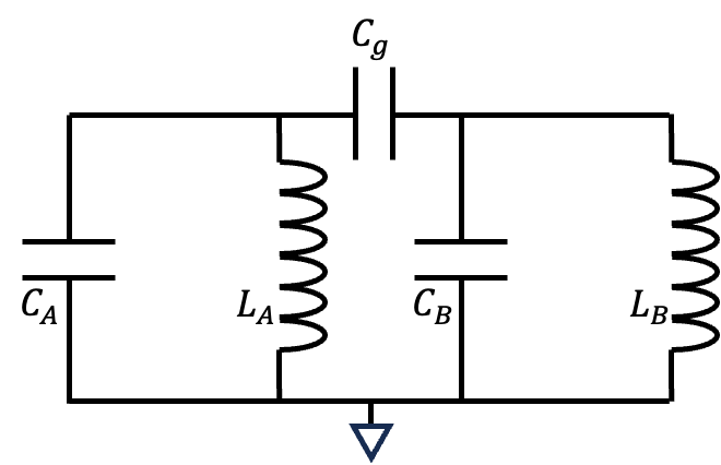
Quantum computation requires coupling between qubits, which can influence the parameters of the qubits. Let us first discuss two linear LC circuits coupled through a capacitor \( C_g \).

\[ \mathcal{L}_{2LC} = \frac{L_A \dot{Q}_A^2}{2} + \frac{L_B \dot{Q}_B^2}{2} - \frac{Q_A^2}{2C_A} - \frac{Q_B^2}{2C_B} - \frac{Q_g^2}{2C_g} \]

The charge \( Q_g \) on the coupling capacitor \( C_g \) can be expressed in terms of \( Q_A \) and \( Q_B \) using the properties of capacitors:

\[ Q_g = C_g (V_A - V_B) = C_g \left( \frac{Q_A}{C_A} - \frac{Q_B}{C_B} \right) \]

Substituting this into the Lagrangian and simplifying:

\[ \mathcal{L}_{2LC} = \frac{L_A \dot{Q}_A^2}{2} + \frac{L_B \dot{Q}_B^2}{2} - \frac{(C_A + C_g) }{2C_A^2} Q_A^2 - \frac{(C_B + C_g) }{2C_B^2}Q_B^2 + \frac{C_g}{C_A C_B} Q_A Q_B \]

Here, define \( C_{\Sigma A} = \frac{C_A^2}{C_A + C_g} \) and \( C_{\Sigma B} = \frac{C_B^2}{C_B + C_g} \). The canonical momentum is defined as:

\[ \Phi_A = -\frac{\partial \mathcal{L}_{2LC}}{\partial \dot{Q}_A} = -L_A \dot{Q}_A \quad \rightarrow \quad \dot{Q}_A = -\frac{\Phi_A}{L_A} \]

The Hamiltonian can then be expressed as:

\[ \bar{\mathcal{H}}_{2LC} = \frac{\Phi_A^2}{2L_A} + \frac{Q_A^2}{2C_{\Sigma A}} + \frac{\Phi_B^2}{2L_B} + \frac{Q_B^2}{2C_{\Sigma B}} - \frac{C_g}{C_A C_B} Q_A Q_B \]

Moving to canonical quantization:

\[ \begin{aligned} &a_{\Sigma A} = \sqrt{\frac{1}{2\hbar} \sqrt{\frac{L_A}{C_{\Sigma A}}}} \left(\sqrt{\frac{C_{\Sigma A}}{L_A}} \Phi_A + iQ_A \right) \\ &a_{\Sigma A}^\dagger = \sqrt{\frac{1}{2\hbar} \sqrt{\frac{L_A}{C_{\Sigma A}}}} \left(\sqrt{\frac{C_{\Sigma A}}{L_A}} \Phi_A - iQ_A \right) \end{aligned} \]

Defining the frequencies \( \omega_{\Sigma A} = \frac{1}{\sqrt{L_A C_{\Sigma A}}} \) and \( \omega_{\Sigma B} = \frac{1}{\sqrt{L_B C_{\Sigma B}}} \):

\[ \bar{\mathcal{H}}_{2LC} = \hbar \omega_{\Sigma A} \left(a_{\Sigma A}^\dagger a_{\Sigma A} + \frac{1}{2}\right) + \hbar \omega_{\Sigma B} \left(a_{\Sigma B}^\dagger a_{\Sigma B} + \frac{1}{2}\right) - \hbar \Omega_g \, i(a_{\Sigma A}^\dagger - a_{\Sigma A}) \, i(a_{\Sigma B}^\dagger - a_{\Sigma B}) \]

The coupling strength \( \Omega_g \) is defined as:

\[ \Omega_g = C_g \sqrt{\frac{\omega_{\Sigma A}}{2(C_A + C_g)}} \sqrt{\frac{\omega_{\Sigma B}}{2(C_B + C_g)}} \]

Appendix:Probability Current in Schrödinger Equation Under Electromagnetic Fields

The wavefunction \(\Psi\) of a particle with charge \(q\) satisfies the Schrödinger equation: \[ i\hbar \partial_t \Psi = \frac{\hat{p}^2}{2m} \Psi + V\Psi, \] where the momentum operator \(\hat{p}\) under the influence of an electromagnetic potential \((\phi, \mathbf{A})\) is expressed as (in SI units): \[ \hat{p} = \frac{\hbar}{i} \nabla - q\mathbf{A}. \] Substituting into the Schrödinger equation gives: \[ i\hbar \partial_t \Psi = \frac{1}{2m} \left( \frac{\hbar}{i} \nabla - q\mathbf{A} \right) \left( \frac{\hbar}{i} \nabla \Psi - q\mathbf{A}\Psi \right) + V\Psi. \] Expanding this yields: \[ i\hbar \partial_t \Psi = -\frac{\hbar^2}{2m} \nabla^2 \Psi - \frac{q}{2m} \frac{\hbar}{i} \nabla \cdot (\mathbf{A}\Psi) - \frac{q}{2m} \frac{\hbar}{i} \mathbf{A} \cdot \nabla \Psi + \frac{q^2 A^2}{2m} \Psi + V\Psi. \]

Its conjugate equation is: \[ -i\hbar \partial_t \Psi^* = -\frac{\hbar^2}{2m} \nabla^2 \Psi^* + \frac{q}{2m} \frac{\hbar}{i} \nabla \cdot (\mathbf{A} \Psi^*) + \frac{q}{2m} \frac{\hbar}{i} \mathbf{A} \cdot \nabla \Psi^* + \frac{q^2 A^2}{2m} \Psi^* + V\Psi^*. \]

Multiplying the first equation by \(\Psi^*\) and the second equation by \(\Psi\), and subtracting the two, we get: \[ i\hbar (\Psi^* \partial_t \Psi + \Psi \partial_t \Psi^*) = -\frac{\hbar^2}{2m} (\Psi^* \nabla^2 \Psi - \Psi \nabla^2 \Psi^*) - \frac{q}{2m} \frac{\hbar}{i} \left[ \Psi^* \nabla \cdot (\mathbf{A}\Psi) + \Psi \nabla \cdot (\mathbf{A}\Psi^*) + \Psi^* \mathbf{A} \cdot \nabla \Psi + \Psi \mathbf{A} \cdot \nabla \Psi^* \right]. \] Simplifying: \[ i\hbar \partial_t (\Psi^* \Psi) = -\frac{\hbar^2}{2m} \nabla \cdot (\Psi^* \nabla \Psi - \Psi \nabla \Psi^*) - \frac{q}{2m} \frac{\hbar}{i} \nabla \cdot (2\mathbf{A} \Psi^* \Psi). \]

Dividing by \(i\hbar\), we get: \[ \partial_t (\Psi^* \Psi) = -\nabla \cdot \left[ \frac{\hbar}{2mi} (\Psi^* \nabla \Psi - \Psi \nabla \Psi^*) - \frac{q\mathbf{A}}{m} \Psi^* \Psi \right]. \] Comparing this with the continuity equation: \[ \partial_t \rho + \nabla \cdot \mathbf{J} = 0, \] where \(\rho = \Psi^* \Psi\) is the probability density, we identify the probability current as: \[ \mathbf{J} = \frac{\hbar}{2mi} (\Psi^* \nabla \Psi - \Psi \nabla \Psi^*) - \frac{q\mathbf{A}}{m} \Psi^* \Psi. \]

For charged particles, the current density \(\mathbf{J}_q\) is: \[ \mathbf{J}_q = q \mathbf{J} = q \left[ \frac{\hbar}{2mi} (\Psi^* \nabla \Psi - \Psi \nabla \Psi^*) - \frac{q\mathbf{A}}{m} \Psi^* \Psi \right]. \] If the wavefunction is expressed in terms of the particle density \(n(\mathbf{r})\) and phase \(\theta(\mathbf{r})\) as \(\Psi \sim \sqrt{n(\mathbf{r})} e^{i\theta(\mathbf{r})}\), then: \[ \mathbf{J}_q = q\frac{\hbar}{m} n(\mathbf{r}) \left[ \nabla \theta(\mathbf{r}) - \frac{q\mathbf{A}}{\hbar} \right]. \]

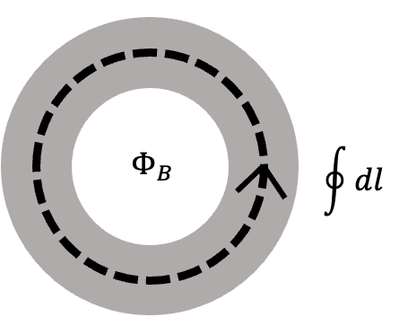
Under topological conditions, and using Stokes' theorem: \[ \int \nabla \times \left[ \nabla \theta(\mathbf{r}) - \frac{q\mathbf{A}}{\hbar} \right] \cdot d\mathbf{S} = \int \nabla \times (\nabla \theta(\mathbf{r})) \cdot d\mathbf{S} - \frac{q}{\hbar} \int (\nabla \times \mathbf{A}) \cdot d\mathbf{S}, \] simplifying to: \[ \oint \nabla \theta(\mathbf{r}) \cdot d\mathbf{l} - \frac{q}{\hbar} \Phi_B = \begin{cases} 0, & \text{if the loop is without a hole}, \\ 2\pi N, & \text{if the loop encloses a hole}. \end{cases} \]

Appendix:Energy Level Corrections Using Perturbation Theory

Using perturbation theory, when \( \mathcal{H} = H_0 + \Delta H \), and the unperturbed eigenstate and eigenvalue are \( |E_0^m\rangle \) and \( E_0^m \), respectively, the perturbed eigenstate and eigenvalue are \( |E^m\rangle \) and \( E^m = E_0^m + \delta E^m \). The energy correction \(\delta E^m\) is given by:

\[ \delta E^m = \langle E_0^m | \Delta H | E_0^m \rangle = \langle E_0^m | \left[-\frac{\hbar^2}{96C} \left(\frac{\pi}{\Phi_0}\right)^2 (a^\dagger + a)^4\right] | E_0^m \rangle. \]

Complete Derivation

\[ \langle E_0^m | (a^\dagger + a)^4 | E_0^m \rangle = \langle E_0^m | (aa + aa^\dagger + a^\dagger a + a^\dagger a^\dagger)^2 | E_0^m \rangle. \]

Expanding this:

\[ \langle E_0^m | aa(aa + aa^\dagger + a^\dagger a + a^\dagger a^\dagger) + aa^\dagger(aa + aa^\dagger + a^\dagger a + a^\dagger a^\dagger) \] \[ + a^\dagger a(aa + aa^\dagger + a^\dagger a + a^\dagger a^\dagger) + a^\dagger a^\dagger(aa + aa^\dagger + a^\dagger a + a^\dagger a^\dagger) | E_0^m \rangle. \]

Taking the expectation value leaves only terms where \( a \) and \( a^\dagger \) appear in equal powers: